DL 딥러닝 RNN-LSTM(56)

LSTM(Long Short-Term Memory):순환 신경망 의 한 유형으로, 시간적으로 멀리 떨어진 데이터 간의 장기 의존성 학습할 수 있는 능력이 특징

• LSTM의 핵심은 '셀 상태'(cell state)라는 내부 메커니즘을 통해 정보를 장기간 저장하고, 필요한 정보만을 선택적으로 통과시키거나 수정할 수 있는 구조

#1.예제 생성
X = []
Y = []
for i in range(3000):
    lst = np.random.rand(100)
    idx = np.random.choice(100, 2, replace=True)
    zeros = np.zeros(100)
    zeros[idx] = 1
    X.append(np.array(list(zip(zeros, lst))))
    Y.append(np.prod(lst[idx]))

print(X[0], Y[0])
# 출력결과
[[0.         0.67267919]
 [0.         0.85503857]
 [0.         0.27878153]
 [0.         0.34400342]
 [0.         0.07751136]
 [0.         0.3449192 ]
 [0.         0.96053807]
 [0.         0.31499018]
 
 
 
 
 
 
 #2. FNN으로 풀어보기
# RNN으로 한 번 풀어보자
model = tf.keras.Sequential([
    tf.keras.layers.SimpleRNN(units=30, return_sequences=True, input_shape =[100,2]),
    tf.keras.layers.SimpleRNN(units=30),
    tf.keras.layers.Dense(1)
])

model.compile(optimizer='adam', loss ='mse')
model.summary()
# 출력
_________________________________________________________________
 Layer (type)                Output Shape              Param #   
=================================================================
 simple_rnn_6 (SimpleRNN)    (None, 100, 30)           990       
                                                                 
 simple_rnn_7 (SimpleRNN)    (None, 30)                1830      
                                                                 
 dense_2 (Dense)             (None, 1)                 31      
 
 
 
 #3. 훈련 (epochs)
 # 훈련
X = np.array(X)
Y = np.array(Y)

history = model.fit(X[:2560], Y[:2560], epochs=100, validation_split = 0.2)


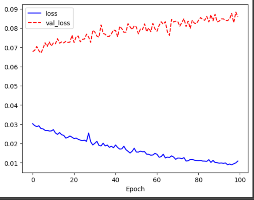
#4. 결과 엉망
 import matplotlib.pyplot as plt
%matplotlib inline

plt.plot(history.history['loss'], 'b-', label = 'loss')
plt.plot(history.history['val_loss'], 'r--', label = 'val_loss')
plt.xlabel('Epoch')
plt.legend()
plt.show()
 

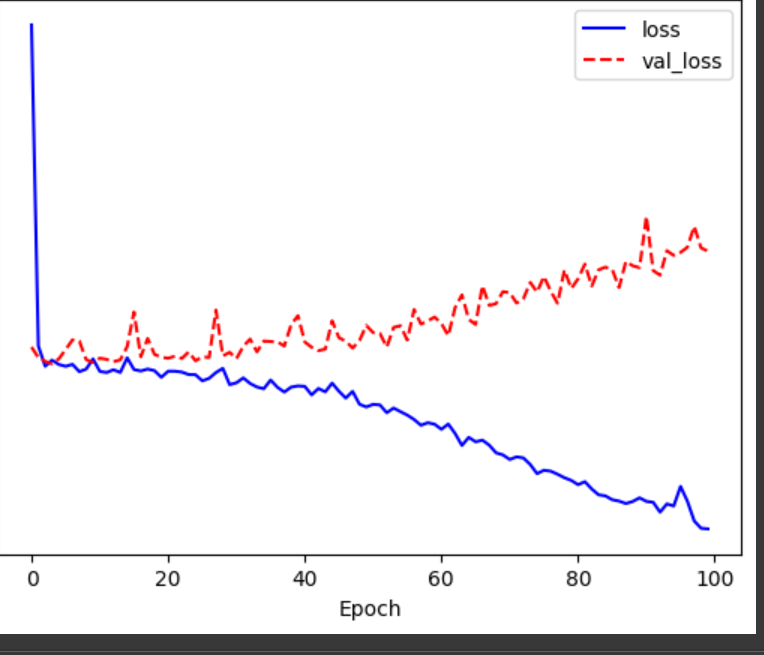
동일하게 훈련 해보기

X = np.array(X)
Y = np.array(Y)

history = model.fit(X[:2560], Y[:2560], epochs=100, validation_split = 0.2)




#시각화
# 다시 시각화
plt.plot(history.history['loss'], 'b-', label='loss')
plt.plot(history.history['val_loss'], 'r--', label = 'val_loss')
plt.xlabel('Epoch')
plt.legend()
plt.show()