
MNIST 딥러닝
NumPy 로 처음부터 손으로 쓴 숫자 이미지를 인식할 수 있도록 딥러닝하는 방법을 살펴본다.
이 딥러닝 모델은 MNIST 데이터 세트로 0 ~ 9 까지의 숫자를 분류하는 벙법을 학습한다. 데이터 세트에는 60,000개의 훈련용 이미지와 10,000개의 테스트 이미지 및 해당 레이블이 포함되어 있다.
이미지 입력 및 해당 레이블(지도학습)을 기반으로한 신경망은 순전파 및 역전파(역방향 모드)를 사용하여 기능을 학습하도록 훈련시킨다.
모듈
NumPy 외에도 데이터 로드 및 처리를 위해서 다음 묘듈을 사용한다.
urllib: URL 처리용request: URL 읽기용gzip: gzip 파일 압축 해제용pickle피클 파일 형식으로 작업Matplotlib데이터 시각화
MNIST 데이터셋 불러오기
Yann에 저장된 압축된 MNIST 데이터셋 파일을 다운한다.
그 후 파이썬 모듈을 사용해 NumPy 배열 유형의 4개 파일로 변환한다.
- MNIST 데이터셋의 학습/테스트 이미지/레이블 이름을 저장
data_sources = {
    "training_images": "train-images-idx3-ubyte.gz",   # 60,000 training images.
    "test_images": "t10k-images-idx3-ubyte.gz",        # 10,000 test images.
    "training_labels": "train-labels-idx1-ubyte.gz",   # 60,000 training labels.
    "test_labels": "t10k-labels-idx1-ubyte.gz"         # 10,000 test labels.
}- 데이터를 로드한다. 저장되어 있는 것을 확인해보자.
Downloading file: train-images-idx3-ubyte.gz
Downloading file: t10k-images-idx3-ubyte.gz
Downloading file: train-labels-idx1-ubyte.gz
Downloading file: t10k-labels-idx1-ubyte.gz- 4개 파일의 압축을 풀고 4개의
ndarrays에 저장한다.
각 원본 이미지 크기는 28x28이고 신경망은 일반적으로 1D 벡터 입력을 예상한다.
mnist_dataset = {}

# 이미지
for key in ("training_images", "test_images"):
    with gzip.open(os.path.join(data_dir, data_sources[key]), 'rb') as mnist_file:
        mnist_dataset[key] = np.frombuffer(mnist_file.read(), np.uint8, offset=16).reshape(-1, 28*28)
# 레이블
for key in ("training_labels", "test_labels"):
    with gzip.open(os.path.join(data_dir, data_sources[key]), 'rb') as mnist_file:
mnist_dataset[key] = np.frombuffer(mnist_file.read(), np.uint8, offset=8)x데이터와y레이블을 표준 표기법으로 사용하기 위해 훈련 및 테스트셋인x_traint,x_test,y_train및y_test로 분할하자.
x_train, y_train, x_test, y_test = (mnist_dataset["training_images"],
                                    mnist_dataset["training_labels"],
                                    mnist_dataset["test_images"],
mnist_dataset["test_labels"])- 훈련과 테스트셋에 대한
(60000, 784)와(10000, 784)와 레이블인(60000,)와(10000,)이 배열의 모양이란 것을 확인할 수 있다.
print('The shape of training images: {} and training labels: {}'.format(x_train.shape, y_train.shape))
print('The shape of test images: {} and test labels: {}'.format(x_test.shape, y_test.shape))
The shape of training images: (60000, 784) and training labels: (60000,)
The shape of test images: (10000, 784) and test labels: (10000,)- 그리고
Matplotlib로 일부 이미지를 검사할 수 있다.
# 훈련셋으로부터의 60,000 번째 이미지 (인덱스 59,999)를
# (784,) 를 (28, 28) 로 적합한 모양으로 만든다.
mnist_image = x_train[59999, :].reshape(28, 28)
# 검은색 배경을 사용하려면 색상 매핑을 그레이스케일로 설정한다.
plt.imshow(mnist_image, cmap='gray')
plt.show()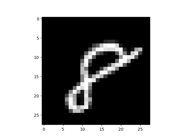
# 훈련셋으로부터 랜덤으로 5개의 이미지
num_examples = 5
seed = 147197952744
rng = np.random.default_rng(seed)

fig, axes = plt.subplots(1, num_examples)
for sample, ax in zip(rng.choice(x_train, size=num_examples, replace=False), axes):
    ax.imshow(sample.reshape(28, 28), cmap='gray')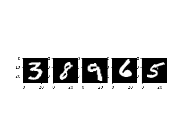
배열로 출력하여 샘플링 이미지를 볼 수도 있다.
60,000 번째 이미지를 8 비트의 배열로 나타낸 것이다.
# 훈련셋으로부터 60,000번째 이미지의 레이블
print(x_train[59999])
print(y_train[59999])
...
0, 0, 38, 48, 48, 22, 0, 0, 0, 0, 0, 0, 0,
0, 0, 0, 0, 0, 0, 0, 0, 0, 0, 0, 0, 0,
0, 62, 97, 198, 243, 254, 254, 212, 27, 0, 0, 0, 0,
...
8데이터 사전 처리하기
신경망은 부동소수점의 텐서(선형 관계) 형식의 입력을 처리할 수 있다.
데이터를 사전 처리할 때, 벡터화 와 부동소수점 변환에 대한 처리를 고려해야 한다.
MNIST 데이터를 이미 벡터화했고, dtype 이 uint8 인 배열로 만들었으니, 다음으로는 float64 와 같은 부동소수점 형식으로 변환해보자.
- 이미지 데이터 정규화 : 데이터의 분포를 표준화하여 신경망 학습 프로세스를 가속화할 수 있는 기능 크기 조정 절차이다.
- 이미지 레이블의 원핫
이미지 데이터를 부동소수점 형식으로 변환
이미지 데이터는 0 ~ 255 사이의 색상이 있는 인코딩된 8비트 정수가 포함돼 있다.
[0, 1] 간격의 부동소수점 배열로 정규화하기 위해 각각의 값에 255 로 나눈다.
- 벡터화된 이미지 데이터에
uint8유형인지 확인
print('The data type of training images: {}'.format(x_train.dtype))
print('The data type of test images: {}'.format(x_test.dtype))
The data type of training images: uint8
The data type of test images: uint8- 배열을 255로 나누어 이미지 데이터 변수를 할당한다. 학습 시간을 줄이기 위해 60,000 및 10,000 개의 이미지의 전체 데이터 집합 중에 1,000 개만 샘플로 포함하자.
training_sample, test_sample = 1000, 1000
training_images = x_train[0:training_sample] / 255
test_images = x_test[0:test_sample] / 255- 이미지 데이터가 부동소수점 형식으로 변경되었는지 확인한다.
print('The data type of training images: {}'.format(training_images.dtype))
print('The data type of test images: {}'.format(test_images.dtype))
The data type of training images: float64
The data type of test images: float64categorical/one-hot 인코딩으로 부동소수점 레이블 변환하기
각 숫자 레이블을 레이블 인덱스를 모두 0 벡터로 포함하여 배치한다.
레이블이 총 10개(0 ~ 9)이므로 배열은 다음과 같다.
array([0., 0., 0., 0., 0., 1., 0., 0., 0., 0.])- 이미지 레이블 데이터가 정수인지 확인
print('The data type of training labels: {}'.format(y_train.dtype))
print('The data type of test labels: {}'.format(y_test.dtype))
The data type of training labels: uint8
The data type of test labels: uint8- 배열에 원핫 인코딩을 수행할 함수를 정의
def one_hot_encoding(labels, dimension=10):
    # 10개의 치수(0 ~ 9) 0 벡터에 대한 단일 원핫 변수를 정의
    one_hot_labels = (labels[..., None] == np.arange(dimension)[None])
    # 인코딩된 원핫 레이블 반환
return one_hot_labels.astype(np.float64)- 레이블을 인코딩하고 값을 새 변수에 할당
training_labels = one_hot_encoding(y_train[:training_sample])
test_labels = one_hot_encoding(y_test[:test_sample])- 데이터 형식이 부동소수점으로 변경되었는지 확인
print('The data type of training labels: {}'.format(training_labels.dtype))
print('The data type of test labels: {}'.format(test_labels.dtype))
The data type of training labels: float64
The data type of test labels: float64- 몇 가지 인코딩된 레이블을 검사
print(training_labels[0])
print(training_labels[1])
print(training_labels[2])
[0. 0. 0. 0. 0. 1. 0. 0. 0. 0.]
[1. 0. 0. 0. 0. 0. 0. 0. 0. 0.]
[0. 0. 0. 0. 1. 0. 0. 0. 0. 0.]원본과 비교해보자.
print(y_train[0])
print(y_train[1])
print(y_train[2])
5
0
4처음부터 작은 신경망 구축하고 훈련
이제 NumPy 에서 간단한 딥러닝 모델의 구성요소를 구성하고 정확도로 MNIST 데이터 집합에서 숫자를 식별하는 법을 학습하도록 훈련한다.
NumPy 를 갖춘 신경망 빌딩 블록
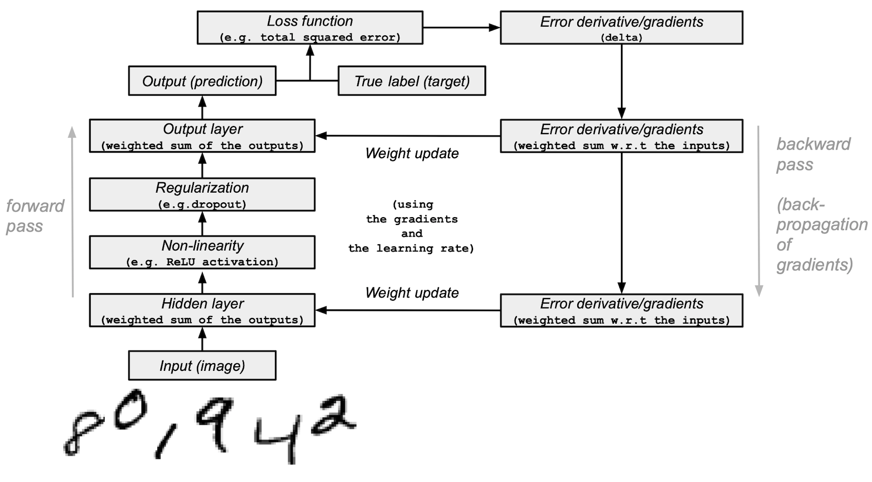
모델 아키텍처 및 교육 요약
다음은 신경망 모델의 아키텍처 및 학습 프로세스 요약이다.
모델을 구성하고 테스트 시작
- 새로운 난수 생성기를 만들어 재현성을 위한 시드를 제공한다.
seed = 884736743
rng = np.random.default_rng(seed)- 히든 레이어의 경우, 순전파를 위한 ReLU 활성화 함수와 역전파 중 사용될 ReLU 의 유도체를 정의
# 입력이 양이면 반환하고 그렇지 않으면 0이면 반환하는 ReLU를 정의
def relu (x):
    return (x>=0) * x

# 양의 입력에 대해 1을, 그렇지 않으면 0을 반환하는 ReLU 기능의 파생 모델을 설정
def relu2deriv(output):
return output >= 0- 다음과 같이 하이퍼매개변수의 특정 기본 값을 설정한다.
learning_rate = 0.005
epochs = 20
hidden_size = 100
pixels_per_image = 784
num_labels = 10- 히든 레이어에 사용되는 가중치 벡터를 임의값으로 초기화
weights_1 = 0.2 * rng.random((pixels_per_image, hidden_size)) - 0.1
weights_2 = 0.2 * rng.random((hidden_size, num_labels)) - 0.1- 신경망의 학습 실험을 설정하고 교육을 시작시킨다.
# 테스트셋 손실과 시각화를 위한 정확한 예측을 저장
store_training_loss = []
store_training_accurate_pred = []
store_test_loss = []
store_test_accurate_pred = []

# 훈련 루프 시작
# 정의된 에포크(반복)의 수에 대한 학습 실험을 실행
for j in range(epochs):

    #################
    #    훈련 단계   #
    #################

    # 손실/오차와 예측 수를 0으로 초기화
    training_loss = 0.0
    training_accurate_predictions = 0

    # 훈련셋의 모든 이미지에 대한 순전파와 역전파를 수행하고 그에 따른 가중치 조정
    for i in range(len(training_images)):
        # 순/역전파 :
        # 1. 입력 레이어:
        #    훈련용 이미지 데이터를 입력으로 초기화
        layer_0 = training_images[i]
        # 2. 히든 레이어:
        #    훈련용 이미지를 랜덤하게 초기화된 가중치를 곱함으로써, 중간 레이어로 가져온다.
        layer_1 = np.dot(layer_0, weights_1)
        # 3. ReLU 활성화 함수를 통해 히든 레이어의 출력을 전달
        layer_1 = relu(layer_1)
        # 4. 정규화를 위한 드롭아웃 함수를 정의
        dropout_mask = rng.integers(low=0, high=2, size=layer_1.shape)
        # 5. 히든 레이어의 출력에 드롭아웃을 적용
        layer_1 *= dropout_mask * 2
        # 6. 출력 레이어:
        #    중간 레이어의 출력을 랜덤하게 초기화된 가중치를 곱하여 최종 레이어로 수집
        #    점수가 10점인 10차원 벡터를 생성
        layer_2 = np.dot(layer_1, weights_2)

        # 역전파:
        # 1. 실제 이미지 레이블과 예측 사이의 오류(손실 함수)를 측정
        training_loss += np.sum((training_labels[i] - layer_2) ** 2)
        # 2. 정확한 예측 카운터 증가시킨다.
        training_accurate_predictions += int(np.argmax(layer_2) == np.argmax(training_labels[i]))
        # 3. 손실/오차를 구분한다.
        layer_2_delta = (training_labels[i] - layer_2)
        # 4. 손실 함수의 경사를 히든 레이어에 다시 전파
        layer_1_delta = np.dot(weights_2, layer_2_delta) * relu2deriv(layer_1)
        # 5. 드롭아웃에 경사 적용
        layer_1_delta *= dropout_mask
        # 6. 학습률과 경사를 곱하여 중간 및 입력 계층에 가중치를 업데이트함
        weights_1 += learning_rate * np.outer(layer_0, layer_1_delta)
        weights_2 += learning_rate * np.outer(layer_1, layer_2_delta)

    # 훈련셋의 손실 및 정확한 예측을 저장
    store_training_loss.append(training_loss)
    store_training_accurate_pred.append(training_accurate_predictions)

    ###################
    #    측정 단계     #
    ###################

    # 각각의 에포크의 테스트셋 성능을 측정한다.

    # 휸련 단계와 달리, 각 이미지(배치)에 대한 수정이 되지 않는다.
    # 그러므로 개별적으로 각 이미지에 루프할 필요가 없는 벡터화된 방법으로 테스트용 이미지에 모델을 적용할 수 있다.

    results = relu(test_images @ weights_1) @ weights_2

    # 실제 레이블과 예측 값 사이의 오차를 측정한다.
    test_loss = np.sum((test_labels - results) ** 2)

    # 테스트셋의 예측 정확도 측정
    test_accurate_predictions = np.sum(
        np.argmax(results, axis=1) == np.argmax(test_labels, axis=1)
    )

    # 테스트셋의 손실 및 정확한 예측을 저장
    store_test_loss.append(test_loss)
    store_test_accurate_pred.append(test_accurate_predictions)

    # 각 에포크에서 오류 및 정확도 메트릭 요약
    print("\n" + \
          "Epoch: " + str(j) + \
          " Training set error:" + str(training_loss / float(len(training_images)))[0:5] + \
          " Training set accuracy:" + str(training_accurate_predictions / float(len(training_images))) + \
          " Test set error:" + str(test_loss / float(len(test_images)))[0:5] + \
          " Test set accuracy:" + str(test_accurate_predictions / float(len(test_images))))
Epoch: 0 Training set error:0.898 Training set accuracy:0.397 Test set error:0.680 Test set accuracy:0.582
Epoch: 1 Training set error:0.656 Training set accuracy:0.633 Test set error:0.606 Test set accuracy:0.641
Epoch: 2 Training set error:0.591 Training set accuracy:0.68 Test set error:0.569 Test set accuracy:0.679
Epoch: 3 Training set error:0.556 Training set accuracy:0.7 Test set error:0.540 Test set accuracy:0.708
Epoch: 4 Training set error:0.534 Training set accuracy:0.732 Test set error:0.525 Test set accuracy:0.729
Epoch: 5 Training set error:0.515 Training set accuracy:0.715 Test set error:0.500 Test set accuracy:0.739
Epoch: 6 Training set error:0.495 Training set accuracy:0.748 Test set error:0.487 Test set accuracy:0.753
Epoch: 7 Training set error:0.483 Training set accuracy:0.769 Test set error:0.486 Test set accuracy:0.747
Epoch: 8 Training set error:0.473 Training set accuracy:0.776 Test set error:0.472 Test set accuracy:0.752
Epoch: 9 Training set error:0.459 Training set accuracy:0.788 Test set error:0.462 Test set accuracy:0.762
Epoch: 10 Training set error:0.464 Training set accuracy:0.769 Test set error:0.462 Test set accuracy:0.767
Epoch: 11 Training set error:0.442 Training set accuracy:0.801 Test set error:0.455 Test set accuracy:0.775
Epoch: 12 Training set error:0.448 Training set accuracy:0.795 Test set error:0.454 Test set accuracy:0.772
Epoch: 13 Training set error:0.438 Training set accuracy:0.787 Test set error:0.452 Test set accuracy:0.778
Epoch: 14 Training set error:0.445 Training set accuracy:0.791 Test set error:0.449 Test set accuracy:0.779
Epoch: 15 Training set error:0.440 Training set accuracy:0.788 Test set error:0.451 Test set accuracy:0.772
Epoch: 16 Training set error:0.437 Training set accuracy:0.786 Test set error:0.452 Test set accuracy:0.772
Epoch: 17 Training set error:0.436 Training set accuracy:0.794 Test set error:0.449 Test set accuracy:0.778
Epoch: 18 Training set error:0.433 Training set accuracy:0.801 Test set error:0.449 Test set accuracy:0.774
Epoch: 19 Training set error:0.429 Training set accuracy:0.785 Test set error:0.436 Test set accuracy:0.784훈련 프로세스는 컴퓨터 처리 능력 및 에포크 수와 같은 여러 요인에 따라 몇 분 정도 걸릴 수 있다. 대기 시간을 줄이려면 에포크 변수를 100에서 더 낮은 숫자로 낮추고 런타임을 재설정(가중치 재설정)한 다음 다시 실행한다.
위 셀을 실행 후 훈련 및 테스트셋 오차/정확도를 시각화할 수 있다.
# 훈련셋 측정 기준
y_training_error = [store_training_loss[i]/float(len(training_images)) for i in range(len(store_training_loss))]
x_training_error = range(1, len(store_training_loss)+1)
y_training_accuracy = [store_training_accurate_pred[i]/ float(len(training_images)) for i in range(len(store_training_accurate_pred))]
x_training_accuracy = range(1, len(store_training_accurate_pred)+1)

# 테스트셋 측정 기준
y_test_error = [store_test_loss[i]/float(len(test_images)) for i in range(len(store_test_loss))]
x_test_error = range(1, len(store_test_loss)+1)
y_test_accuracy = [store_training_accurate_pred[i]/ float(len(training_images)) for i in range(len(store_training_accurate_pred))]
x_test_accuracy = range(1, len(store_test_accurate_pred)+1)

# 시각화
fig, axes = plt.subplots(nrows=1, ncols=2, figsize=(15, 5))
axes[0].set_title('Training set error, accuracy')
axes[0].plot(x_training_accuracy, y_training_accuracy, label = "Training set accuracy")
axes[0].plot(x_training_error, y_training_error, label = "Training set error")
axes[0].set_xlabel("Epochs")
axes[1].set_title('Test set error, accuracy')
axes[1].plot(x_test_accuracy, y_test_accuracy, label = "Test set accuracy")
axes[1].plot(x_test_error, y_test_error, label = "Test set error")
axes[1].set_xlabel("Epochs")
plt.show()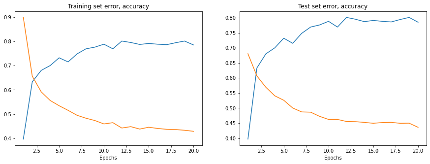
훈련 및 테스트 중 모델이 도달하는 정확도는 다소 그럴듯 하지만 오차률이 상당히 높을 수도 있다.
이에 대한 솔루션은 다음과 같다.
다음 단계
신경망 모델을 더욱 향상시키고 최적화하기 위해 다음을 고려할 수 있다.
