❗머신러닝 프로세스 : 데이터 가공/변환 → 모델 학습/예측 → 평가
❗넘파이 ndarray, 판다스 dataframe
❗reshape(-1, 1) 열을 1개로 만들고, 행은 알아서 조정됨
❗x[:, 1] 모든 행을 가져오는데, 1번 인덱스의 열(그니까 두번째)에서만 가져오기
01. 평가
-
머신러닝 모델은 여러 가지 방법으로 예측 성능을 평가할 수 있다.
-
성능 평가 지표: 모델이 회귀인지, 분류인지에 따라 여러 종류로 나뉜다.
- 회귀: 실제값과 예측값의 오차 평균값에 기반한다. = 예측 오차를 가지고 정규화 수준 재가공
- 분류: 단순히 정확도만 가지고 판단했다간 잘못된 평가 결과에 빠질 수 있다.
02. 분류 모델 평가
-
단순히 정확도만 가지고 판단했다간 잘못된 평가 결과에 빠질 수 있다.
-
분류는 2개의 결과값만을 가지는 이진 분류, 그 이상의 결정 클래스 값을 가지는 멀티 분류로 나뉠 수 있다.
-
특히 0과 1로 결정값이 한정되는 이진 분류의 성능 평가 지표에 대해서 공부한다.
1) 정확도 (Accuracy)
-
실제 데이터에서 예측 데이터가 얼마나 같은지 판단하는 지표

-
이진 분류에서, 데이터의 구성에 따라 모델의 성능을 왜곡할 수 있으므로 단독으로 사용하지는 않는다.
-
불균형한 레이블 데이터 세트에서는 성능 수치로 사용해서는 안 된다.
-
Sklearn의
BaseEstimator: 상속받으면 Estimator를 customize해서 생성 가능
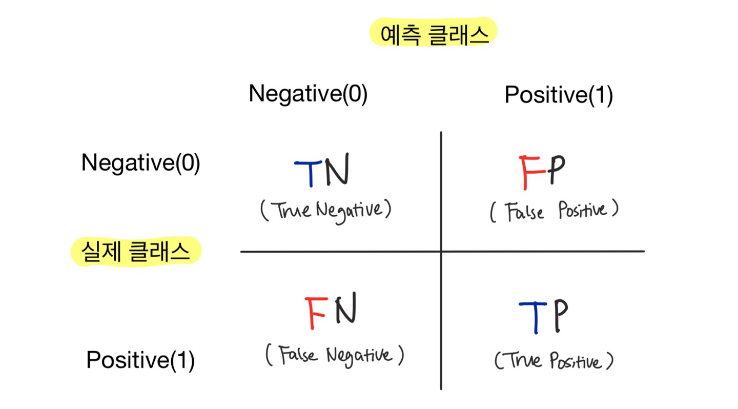
2) 오차 행렬 (Confusion Matrix)
-
학습된 분류 모델이 예측을 수행하면서 얼마나 헷갈리고 있는지도 함께 보여주는 지표
→ 이진 분류의 예측 오류 & 어떠한 유형의 예측 오류가 발생하고 있는지 나타낸다. -
이진 분류에서 성능 지표로 잘 활용된다.
-
4분면 행렬에서 실제 레이블 클래스 값과 예측 레이블 클래스 값이 어떤 유형으로 매핑되는지를 나타낸다.
-
Sklearn에서
confusion_matrix()API를 이용해 오차 행렬을 구할 수 있다. -
오차 행렬 상에서의 정확도는 True에 해당하는 값에 의해서만 좌우되므로 다음과 같이 표현 가능하다.
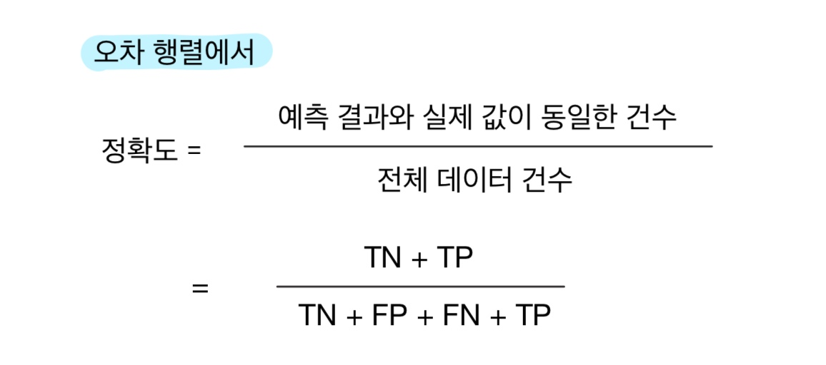
-
일반적으로, 불균형한 레이블 클래스를 가지는 이진 분류 모델에서는 많은 데이터 중에서 중점적으로 찾아야 하는 매우 적은 수의 결과값에 Positive를 설정해 '1'값을 부여하는 경우가 많다.
❗결론 : 정확도는 불균형한 데이트 세트에서 분류 모델의 성능 지표로 사용되기 어렵다.
3) 정밀도 (Precision), 재현율 (Recall)
-
정밀도와 재현율은 'Positive' 데이터 세트의 예측 성능에 초점을 맞춘 평가 지표이다.
-
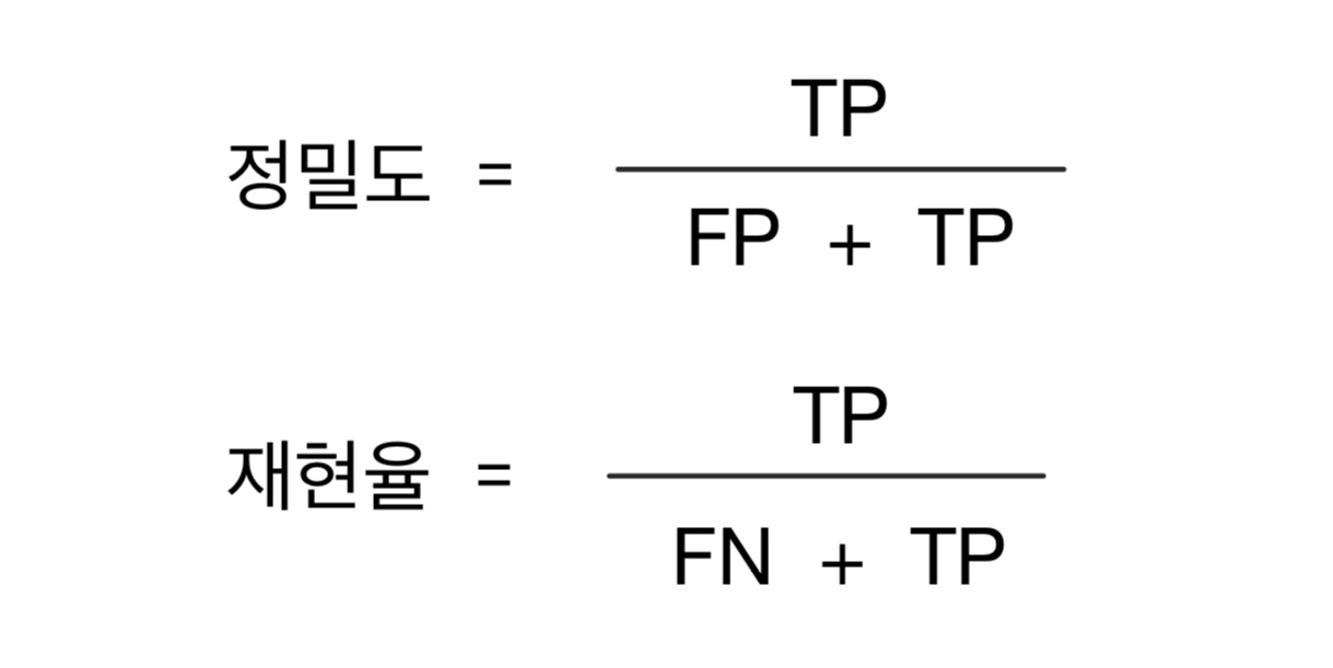
정밀도와 재현율의 공식은 다음과 같다.
-
정밀도: 예측을 Positive로 한 대상 중에 예측 값이 실제 값과 Positive로 일치한 데이터의 비율, 분모는 예측을 Positive로 한 모든 건수가 된다. Positive 예측 성능을 정밀하기 측정하기 위한 평가 지표로서 '양성 예측도'라고도 불린다.
-
재현율: 실제 값이 Positive인 대상 중에 예측 값이 실제 값과 Positive로 일치한 데이터의 비율, 분모는 실제 값이 Positive인 모든 건수가 된다. '민감도' 또는 'TPR (True Positive Rate)'라고도 불린다.
-
재현율이 중요 지표인 경우는 실제 Positive 데이터를 Negative로 잘못 판단하게 됐을 때 큰 영향이 발생하는 경우이다.
e.g. 암 판단 모델 : 실제 암 환자를 Positive가 아닌 Negative로 판단 시 큰 위험이 따른다.
e.g. 금융 사기 적발 모델 : 실제 금융 사기 건을 Negative로 잘못 판단하면 큰 손해가 발생한다. -
보통 재현율이 정밀도보다 상대적으로 중요하지만,
실제 Negative인 데이터 예측을 Positive로 잘못 판단 시 큰 영향이 있을 경우, 정밀도가 상대적으로 더 중요한 지표이다. -
Sklearn에서 정밀도 계산을 위해
precision_score(), 재현율 계산을 위해recall_score()API를 사용할 수 있다. -
정밀도/재현율 트레이드오프 (Tradeoff)
- 정밀도와 재현율은 상호 보완적인 평가 지표이기 때문에 어느 한 쪽을 강제로 높이면 다른 한 쪽의 수치는 떨어지기 쉽다.
-
Sklearn은 개별 데이터별로 예측 확률을 반환하는 메서드인
predict_proba()를 제공한다.- 해당 메서드는 학습이 완료된 Sklearn Classifier 객체에서 호출 가능
- 테스트 피처 데이터 세트를 파라미터로 입력 → 테스트 피처 레코드의 개별 클래스 예측 확률을 반환
- 정해진 임곗값(e.g. 0.5)을 만족하는 ndarray의 칼럼 위치를 최종 예측 클래스로 결정
-
Binarizer(): Binarizer 객체의fit_transform()을 이용해 넘파이의 ndarray를 입력하면, 입력된 ndarray의 값을 지정된 threshold보다 같거나 작으면 0으로, 크면 1로 변환해 리턴한다.
from sklearn.preprocessing import Binarizer

X = [[1, -1, 2], [2, 0, 0], [0, 1.1, 1.2]]

# X의 각 원소들이 threshold(1.1)값보다 같거나 작으면 0, 크면 1 리턴
binarizer = Binarizer(threshold=1.1)
print(binarizer.fit_transform(X))- 임곗값(threshold)을 낮추면 재현율이 올라가고 정밀도가 떨어지는 경향이 나타난다. 더 너그럽게 Positive로 예측하기 때문에 True값이 많아지게 된다.
# 테스트할 임곗값들
thresholds = [0.4, 0.45, 0.5, 0.55, 0.6]

def get_eval_by_threshold(y_test, pred_proba_c1, thresholds):
    for custom_threshold in thresholds:
        binarizer = Binarizer(threshold=custom_threshold).fit(pred_proba_c1)
        custom_predict = binarizer.transform(pred_proba_c1)
        print('임곗값:', custom_threshold)
        get_clf_eval(y_test, custom_predict)

get_eval_by_threshold(y_test, pred_proba[:, 1].reshape(-1, 1), thresholds)- Sklearn에서 이와 유사한
precision_recall_curve()API를 제공한다.- 입력 파라미터 :
y_true실제 클래스값 배열,probas_predPositive 칼럼의 예측 확률 배열 - 반환 값 : 정밀도, 재현율
- 대체로 임곗값이 증가할수록 정밀도는 동시에 높아지나 재현율 값은 낮아짐
- 입력 파라미터 :
from sklearn.metrics import precision_recall_curve

# 레이블 값이 1일 때의 예측 확률 추출
pred_proba_class1 = lr_clf.predict_proba(X_test)[:, 1]


# 실제값 데이터 세트와, 레이블 값이 1일 때의 예측 확률을 precision_recall_curve 인자로 입력
precisions, recalls, thresholds = precision_recall_curve(y_test, pred_proba_class1)
print('반환된 분류 결정 임곗값 배열의 Shape:', thresholds.shape)

# 반환된 임계값 로우(행)가 147건이므로 샘플로 10건만 추출하되, 임곗값을 15 step으로 추출
thr_index = np.arange(0, thresholds.shape[0], 15)
print('샘플 추출을 위한 임계값 배열의 index 10개:', thr_index)
print('샘플용 10개의 임곗값: ', np.round(thresholds[thr_index], 2))

# 15 step 단위로 추출된 임계값에 따른 정밀도와 재현율 값
print('샘플 임계값별 정밀도:', np.round(precisions[thr_index], 3))
print('샘플 임계값별 재현율:', np.round(recalls[thr_index], 3))precision_recall_curve()는 정밀도와 재현율의 임곗값에 따른 값 변화를 곡선 형태 그래프로 시각화할 수 있다.
import matplotlib.pyplot as plt
import matplotlib.ticker as ticker
%matplotlib inline

def precision_recall_curve_plot(y_test, pred_proba_c1):

    # 각 값을 ndarray로 추출
    precisions, recalls, thresholds = precision_recall_curve(y_test, pred_proba_c1)

    # X축: threshold값, Y축: 정밀도와 재현율
    plt.figure(figsize=(8, 6))
    threshold_boundary = thresholds.shape[0]

    # 정밀도 그리기
    plt.plot(thresholds, precisions[0:threshold_boundary], linestyle='--', label='precision')
    # 재현율 그리기
    plt.plot(thresholds, recalls[0:threshold_boundary], label='recall')

    # threshold값 X축의 scale을 0.1 단위로 변경
    start, end = plt.xlim()
    plt.xticks(np.round(np.arange(start, end, 0.1), 2))

    # x, y축 label & legend, grid 설정
    plt.xlabel('Threshold value');plt.ylabel('Precision and Recall value')
    plt.legend();plt.grid()
    plt.show()


precision_recall_curve_plot(y_test, lr_clf.predict_proba(X_test)[:, 1])
[output]
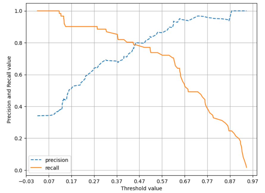
- 정밀도가 100%가 되는 법 : 확실한 기준이 되는 경우(모든 경우를 만족하는 정도의 확실한 경우)에만 Positive로 예측
- 재현율이 100%가 되는 법 : 모든 경우를 Positive로 예측
→ 정밀도와 재현율이 적절하게 조합되어 분류의 종합적인 성능 평가에 사용될 수 있는 평가 지표가 필요하다.
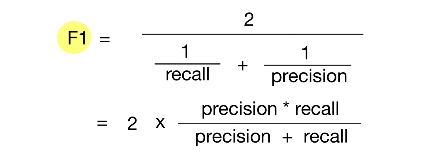
4) F1 스코어
- 정밀도와 재현율을 결합한 지표
- 정밀도와 재현율이 어느 한 쪽으로 치우치지 않는 수치를 나타낼 때 상대적으로 높은 값을 가진다.
- Sklearn에서
f1_score()API를 제공한다.
from sklearn.metrics import f1_score

f1 = f1_score(y_test, pred)
print('F1 스코어: {0:.4f}'.format(f1))- 적용 예시 코드 (임곗값을 변화시키면서 F1 스코어를 포함한 평가 지표 구하기)
def get_clf_eval(y_test, pred):
    confusion = confusion_matrix(y_test, pred)
    accuracy = accuracy_score(y_test, pred)
    precision = precision_score(y_test, pred)
    recall = recall_score(y_test, pred)

    # F1 score 추가
    f1 = f1_score(y_test, pred)

    print('오차 행렬')
    print(confusion)

    # F1 score print 추가
    print('정확도: {0:.4f}, 정밀도: {1:.4f}, 재현율: {2:.4f}, F1: {3:.4f}'.format(accuracy, precision, recall, f1))


thresholds = [0.4, 0.45, 0.5, 0.55, 0.6]
pred_proba = lr_clf.predict_proba(X_test)
get_eval_by_threshold(y_test, pred_proba[:, 1].reshape(-1, 1), thresholds)
5) ROC 곡선과 AUC
- ROC 곡선 (Receiver Operation Characteristics Curve): 머신 러닝의 이진 분류 모델의 예측 성능을 판단하는 중요한 평가 지표
- FPR(False Positive Rate)이 변할 때 TPR(True Positive Rate)이 어떻게 변하는지 나타내는 곡선
- FPR을 X축으로, TPR을 Y축으로 잡는다.
- TPR은 재현율을 나타내며, 민감도를 의미한다. 실제 Positive가 정확이 예측되어야 하는 수준을 나타낸다.
- TNR은 특이성을 의미한다. 실제 Negative가 정확히 예측되어야 하는 수준을 나타낸다.

- Sklearn은 ROC 곡선을 구하기 위해
roc_curve()API를 제공한다.
def roc_cuvre_plot(y_test, pred_proba_c1):

    fprs, tprs, thresholds = roc_curve(y_test, pred_proba_c1)
    plt.plot(fprs, tprs, label='ROC')
    plt.plot([0,1], [0,1], 'k--', label='Random')

    start, end = plt.xlim()
    plt.xticks(np.round(np.arange(start, end, 0.1), 2))
    plt.xlim(0, 1); plt.ylim(0, 1)
    plt.xlabel('FPR( 1 - Specificity )'); plt.ylabel('TPR( Recall )')
    plt.legend()
    plt.show()

roc_curve_plot(y_test, lr_clf.predict_proba(X_test)[:, 1] )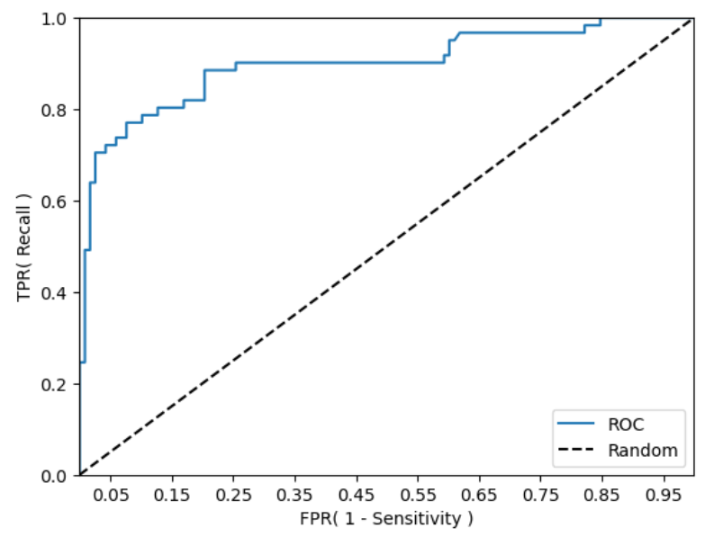
- ROC 곡선 자체는 일반적으로 FPR과 TPR의 변화 값을 보는 데 이용되며, 분류의 성능 지표로 이용되는 것은 ROC 곡선 면적에 기반한 AUC 값으로 결정한다.
- AUC (Area Under Curve) : ROC 곡선 밑의 면적을 구한 것으로 일반적으로 1에 가까울수록 좋은 수치
- AUC 수치가 커지려면 FPR이 작은 상태에서 얼마나 큰 TPR을 얻을 수 있느냐가 관건이다.
from sklearn.metrics import roc_auc_score

pred_proba = lr_clf.predict_proba(X_test)[:, 1]
roc_score = roc_auc_score(y_test, pred_proba)
print('ROC AUC 값: {0:.4f}'.format(roc_score))
보완 & 실습 Part
predict_proba()
- 분류 모델이 각 클래스에 대한 확률을 일일이 출력하는 것
-predict_proba[ : , 1]이진분류 문제에서, 회귀문제를 분류모델을 통해 푸는 방식을 뜻하며 이는 곧 1일 확률을 의미
-predict와 비교
- predict는 모델의 최종적인 예측값을 출력
- predict_proba는 각 클래스의 예측 확률을 출력
(클래스가 3개 라면 0일 확률, 1일 확률, 2일 확률)
train_test_split()
-stratify: 지정한 Data의 비율을 유지하기 위한 설정, 예를 들어, Label Set인 Y가 25%의 0과 75%의 1로 이루어진 Binary Set일 때,stratify=Y로 설정하면 나누어진 데이터셋들도 0과 1을 각각 25%, 75%로 유지한 채 분할된다
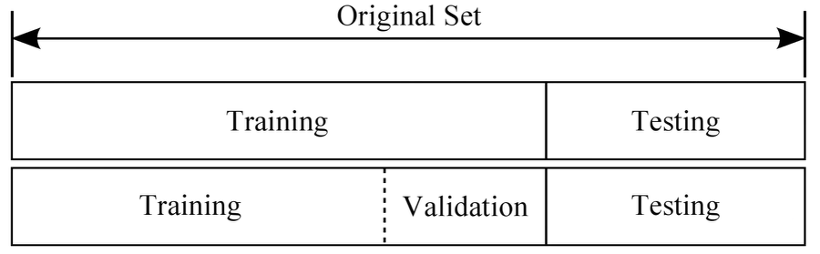
- 데이터셋 나누기
- 일반적으로 Training : Validation : Test = 6 : 2 : 2
- Training set : 모델을 학습하는 데 사용
- Validation set : Training set으로 만들어진 모델의 성능 측정을 위함, Validation set로 가장 성능이 좋았던 모델을 선택
- Test set : 마지막으로 딱 한 번, 해당 모델의 성능을 측정하기 위함
from sklearn.model_selection import train_test_split
train_test_split(arrays, test_size, train_size, random_state, shuffle, stratify)참조
📁 train_test_split() : https://blog.naver.com/PostView.naver?blogId=siniphia&logNo=221396370872
📁 dataset 내용 정리 : https://ganghee-lee.tistory.com/38