Introduction to Deep Neural Networks

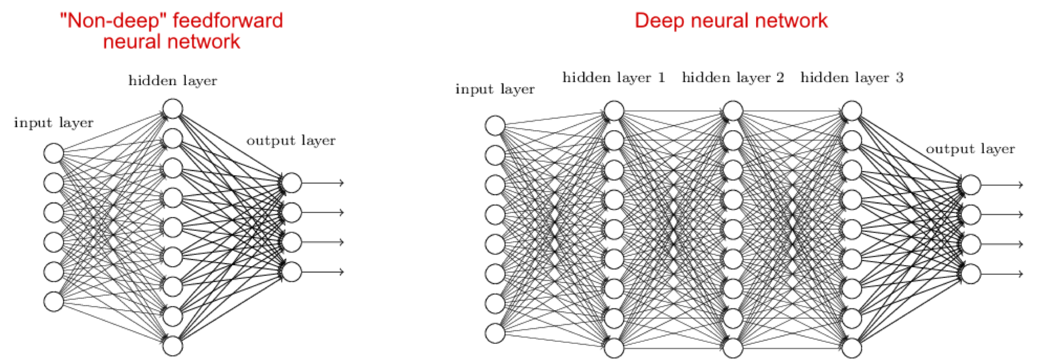
Deep Neural Network (DNN)

• DNN improves accuracy of AI technology by stacking neural network layers
  

Applications of Deep Learning

• Computer Vision
• Natural Language Processing
• Time-Series Analysis
• Reinforcement Learning

Perceptron and Neural Networks

What is Perceptron?

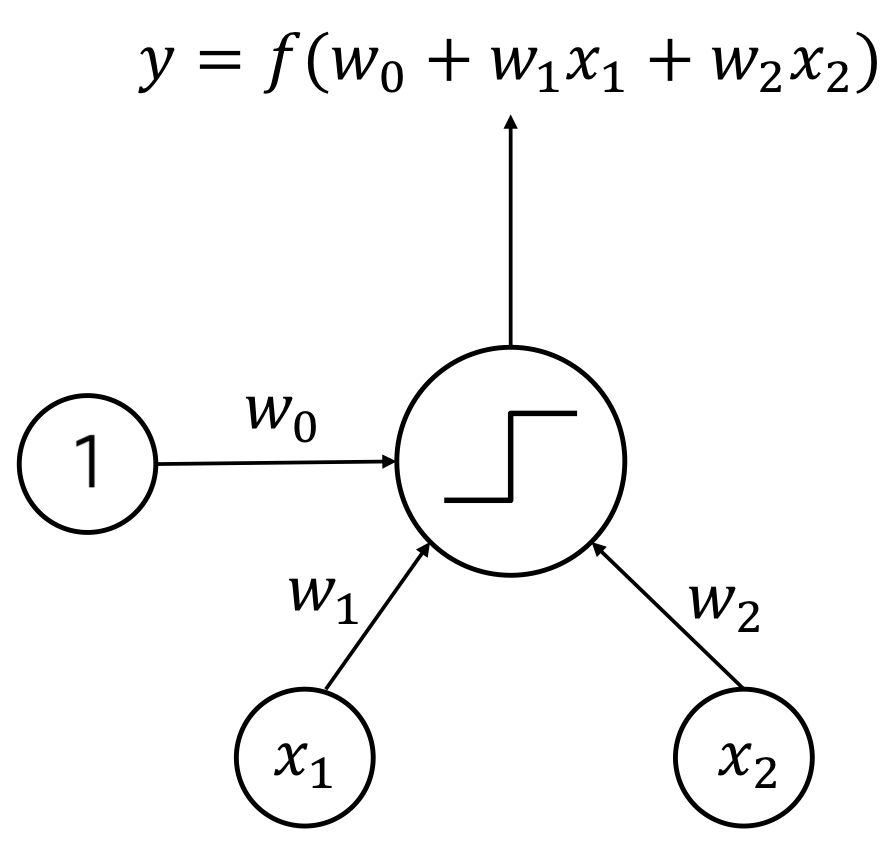
Perceptron

• One kind of neural networks
• Frank Rosenblatt devised in 1957
• Linear Classifier
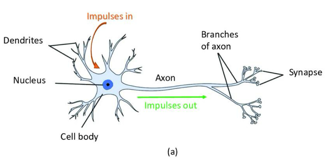
• Similar with structure of a neuron
  

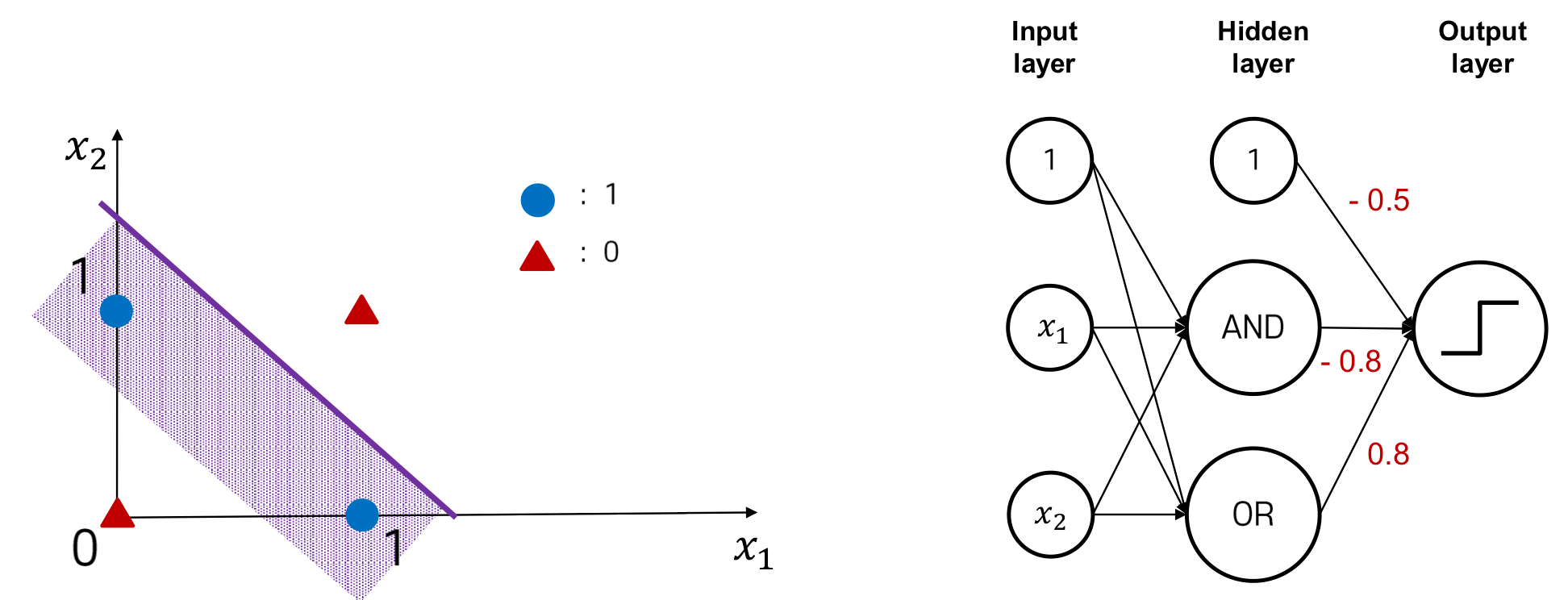
Multi-Layer Perceptron for XOR Gate

Is it possible to solve a XOR problem using a single layer perceptron?
→ No. Single layer perceptron can only solve linear problem. XOR problem is non-linear

But if we use two-layer perceptron, we can solve XOR problem
→ This model is called multi-layer perceptron

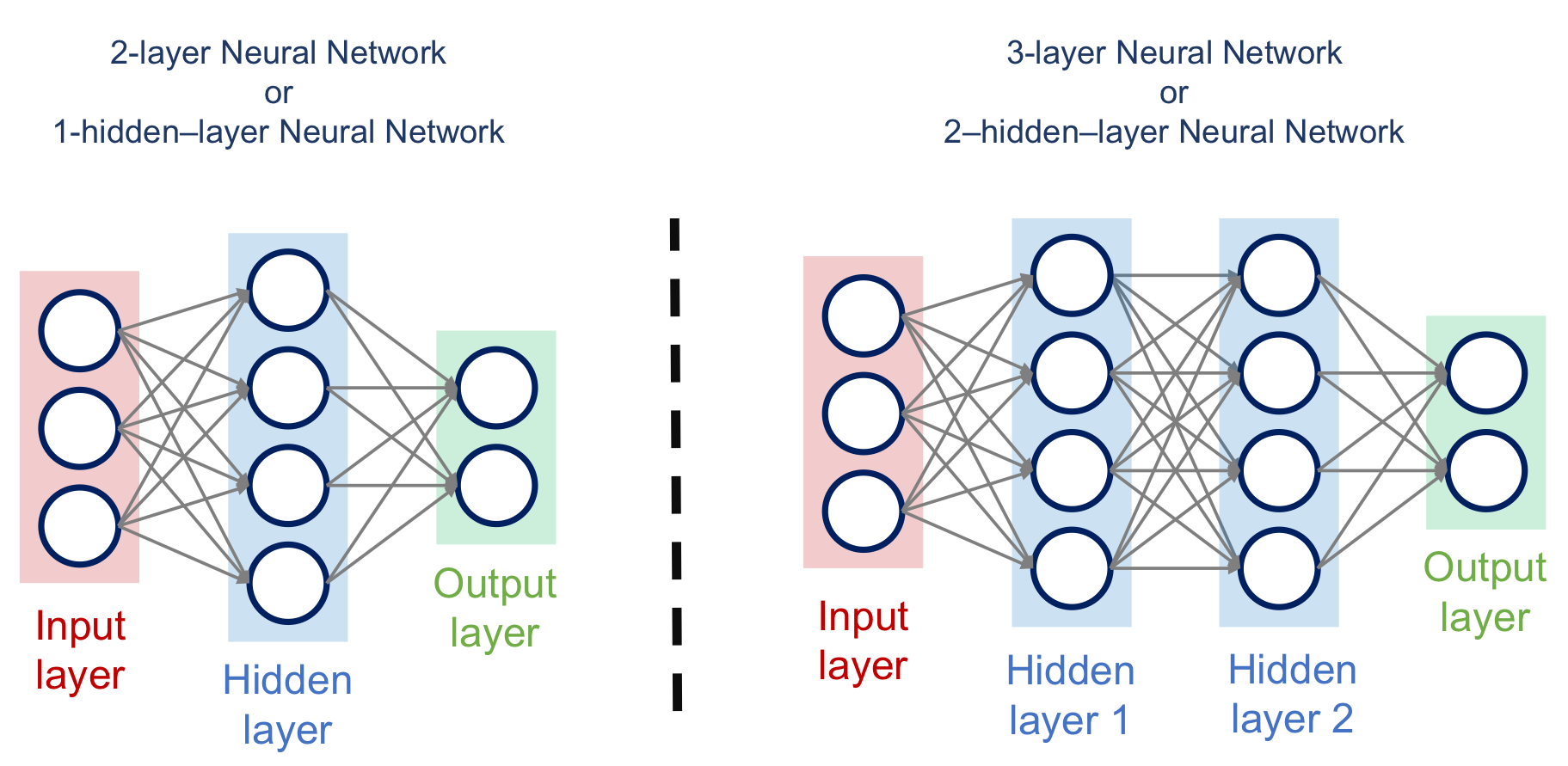
Hidden Layer

Forward Propagation

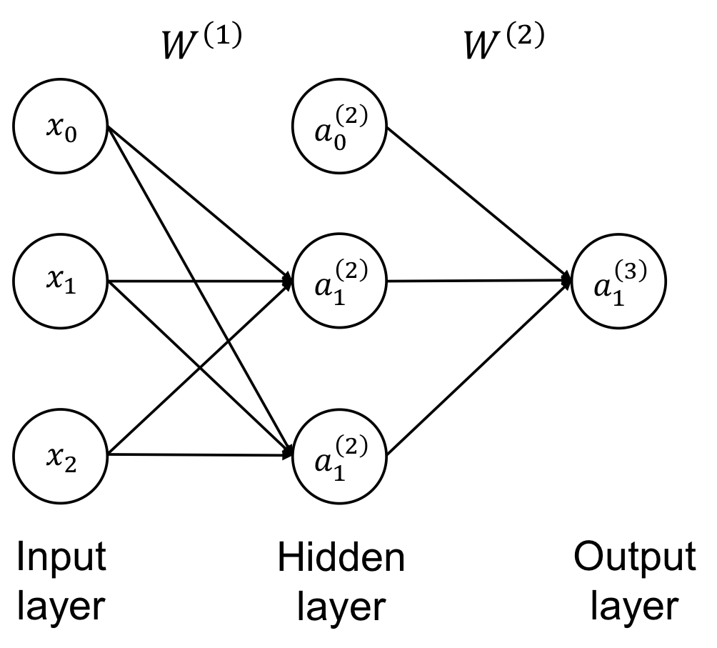
• $a_j^{(i)}$ : "Activation" of the i-th unit in the j-th layer
  → $j$는 layer, $i$는 layer내에 몇 번째 노드냐
• $W^{(j)}$ : "Weight Matrix" mapping from the j-th layer to the (j+1)-th layer.

Linear Layer

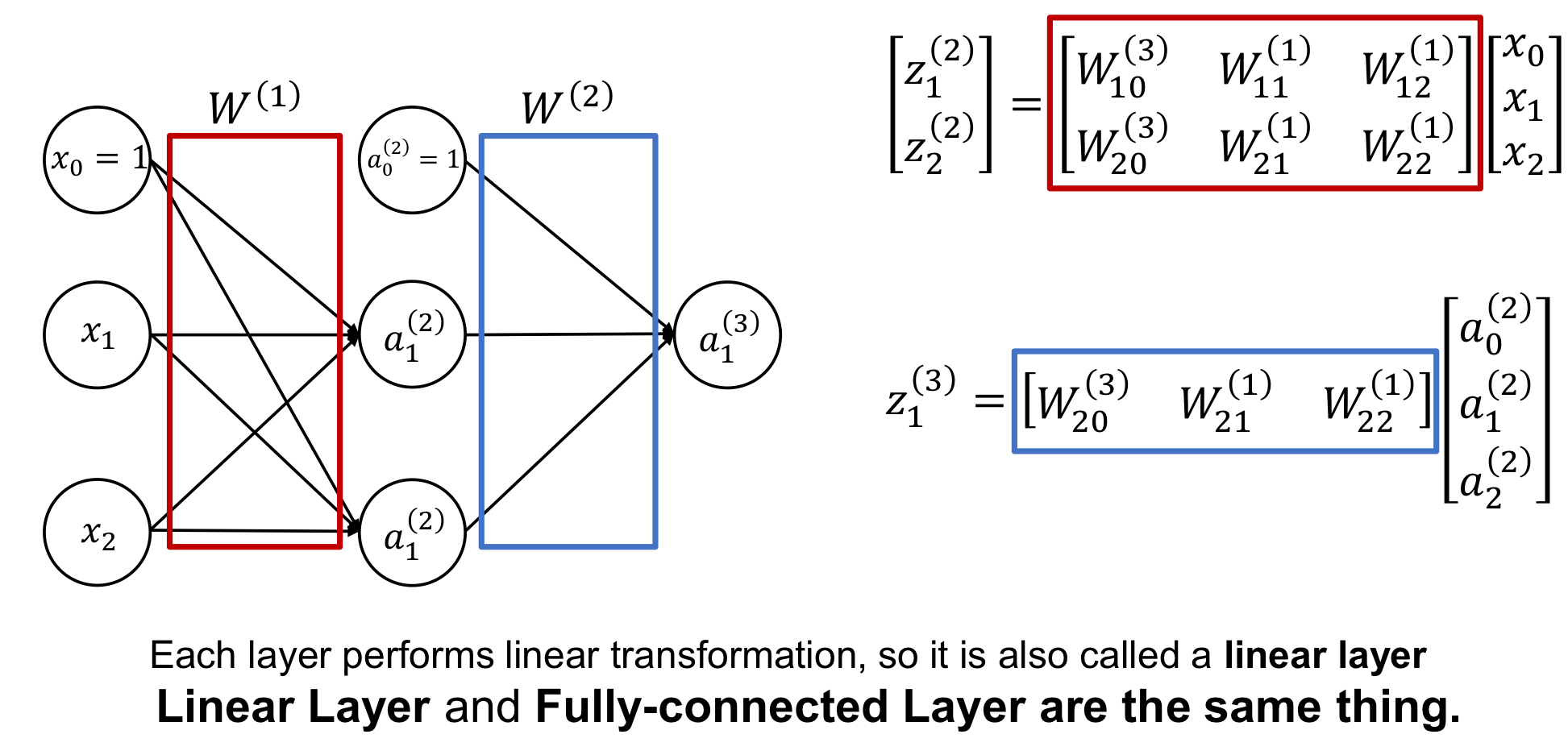
Each layer performs linear transformation, so it is also called a linear layer.
Linear Layer and Fully-connected Layer are the same thing.

Training Neural Networks

Training Neural Networks via Gradient Descent

Given the optimization problem, $min_{W}L(w)$, where $W$ is the neural network parameters, we optimize $W$ using gradient descent approach:

Q: What is the trajectory along which we converge towards the minimum with SGD?
→ Veryslow progress along flat direction, jitter along steep one

Backpropagation to Compute Gradient in Neural Networks

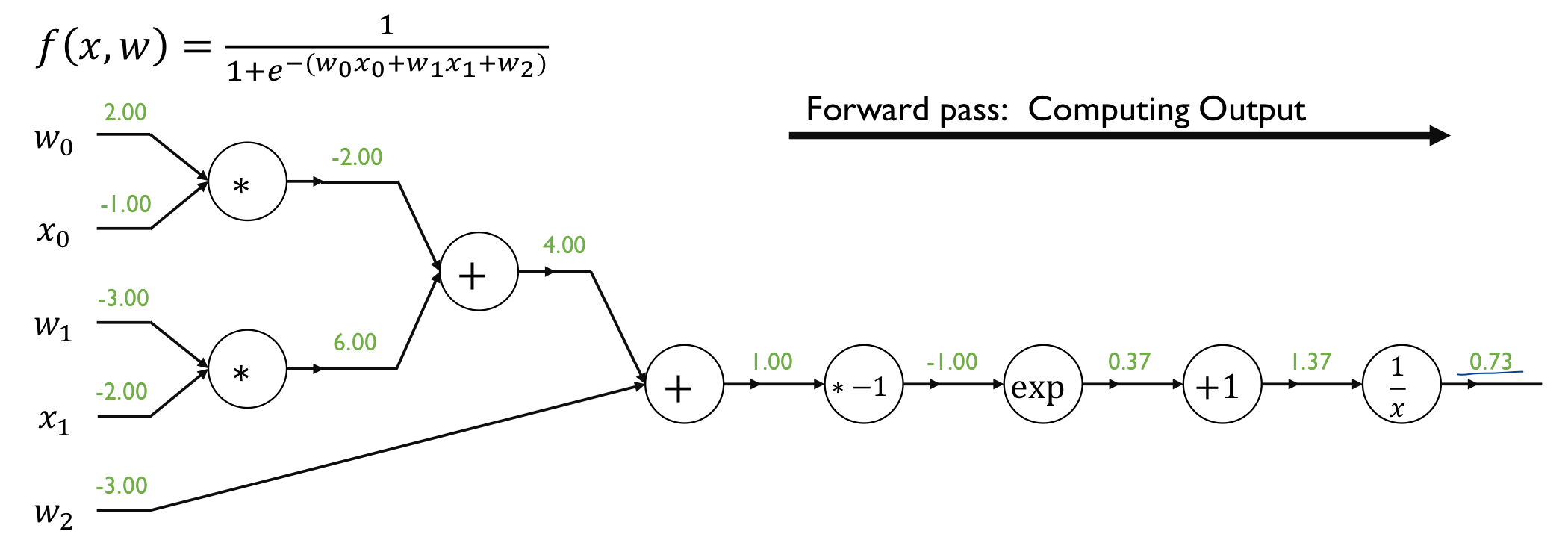
1. given an input data item, compute the loss function value via Forward Propagation
2. compute the gradient with respect to each neural network parameter via Backpropagation
3. update the parameters using gradient descent algorithm
   
   
   
   
   
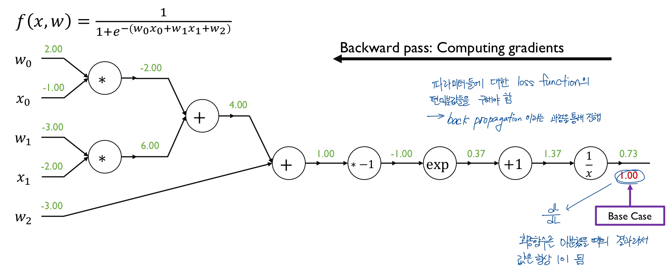
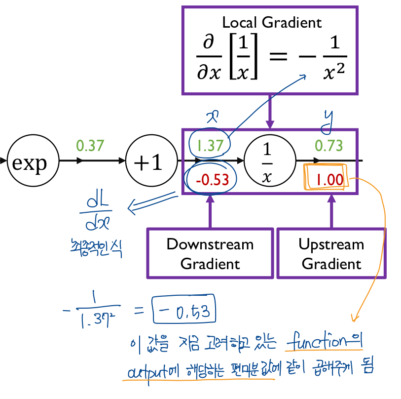
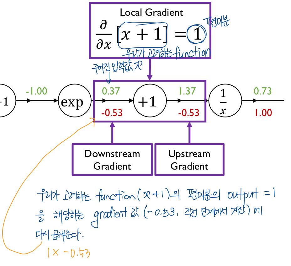
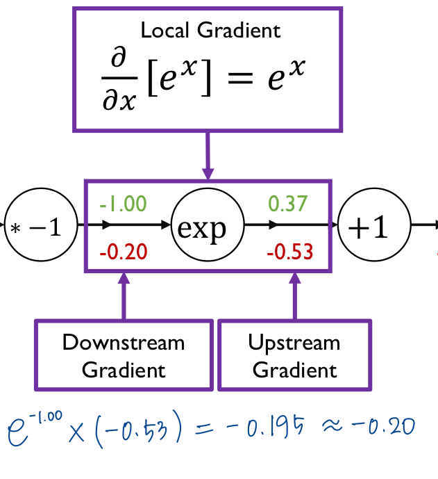
   이런 식으로 계산해 주면 된다.
   중간에 계산한 gradient들은 중간 결과물로서 결과들이 계산되지만 직접적인 gradient descentd에는 사용되지 않는 노드들이다.
   $w_0, w_1, w_2$ 가 갱신되는 노드들이다.

Sigmoid Activation

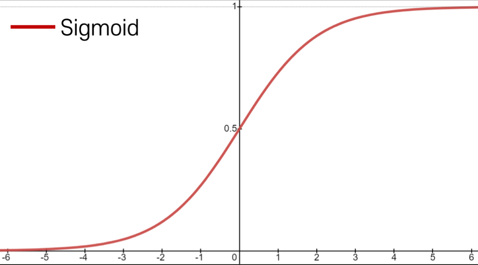
Sigmoid

• Maps real numbers in $(-\infty, \infty)$ into a range of $[0,1]$
• gives a probabilistic interpretation

Problems of Sigmoid Activation

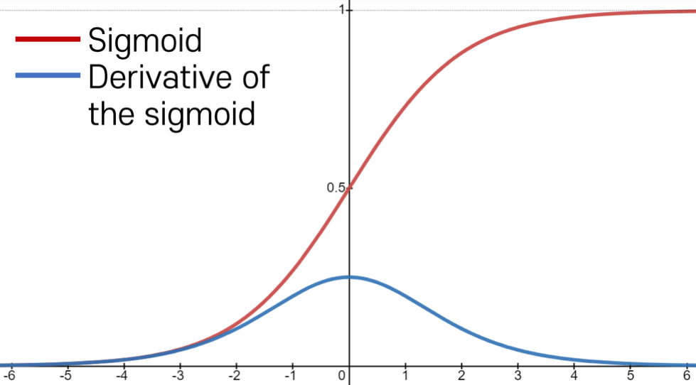
• Saturated neurons kills the gradient
• The gradient value $\sigma(x) \le \frac{1}{4}$, which decreases the gradient during backpropagation, i.e., causing a gradient vanishing problem
  → 역전파를 진행할수록 gradient 값이 점점 작아지는 양상을 보임
  → gradient vanishing problem

Tanh Activation

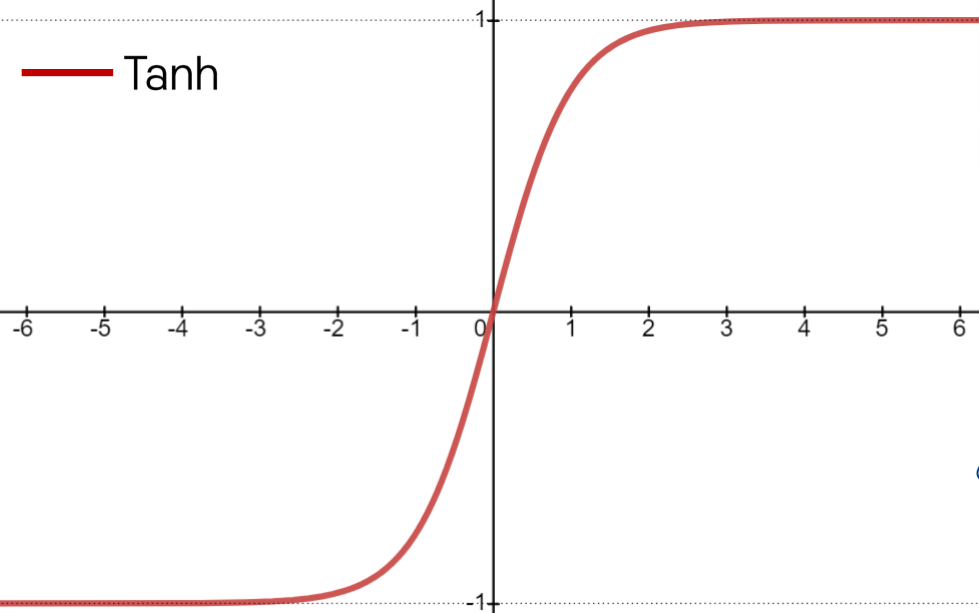
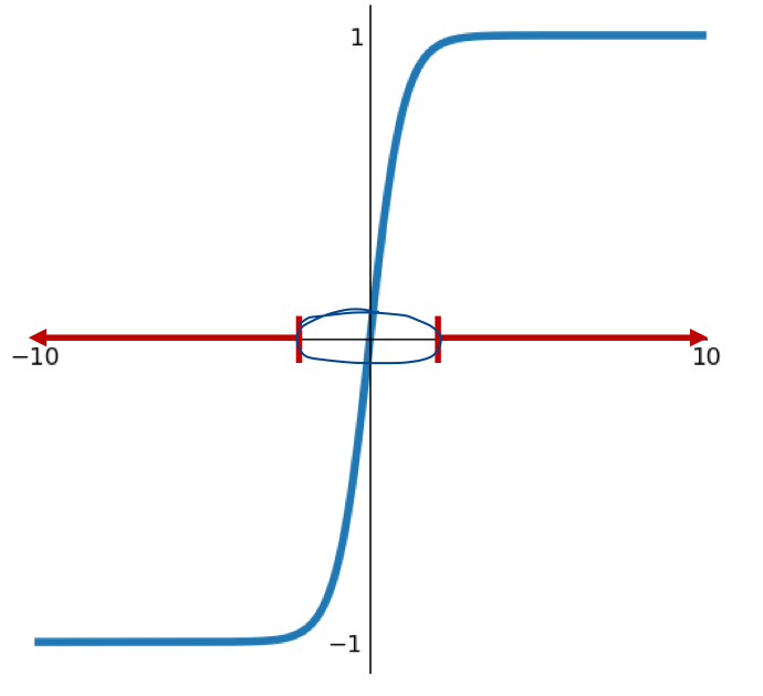
Tanh

• $tanh(x) = 2 \times sigmoid(x) - 1$
• Squashes numbers to range $[-1,1]$

Strength

• Zero-centered (average is 0)

Weakness

• Still kills gradients when saturated, i.e., still causing a gradient vanishing problem
  $rarr; 값이 -1 ~ 1이기 때문에

ReLU Activation

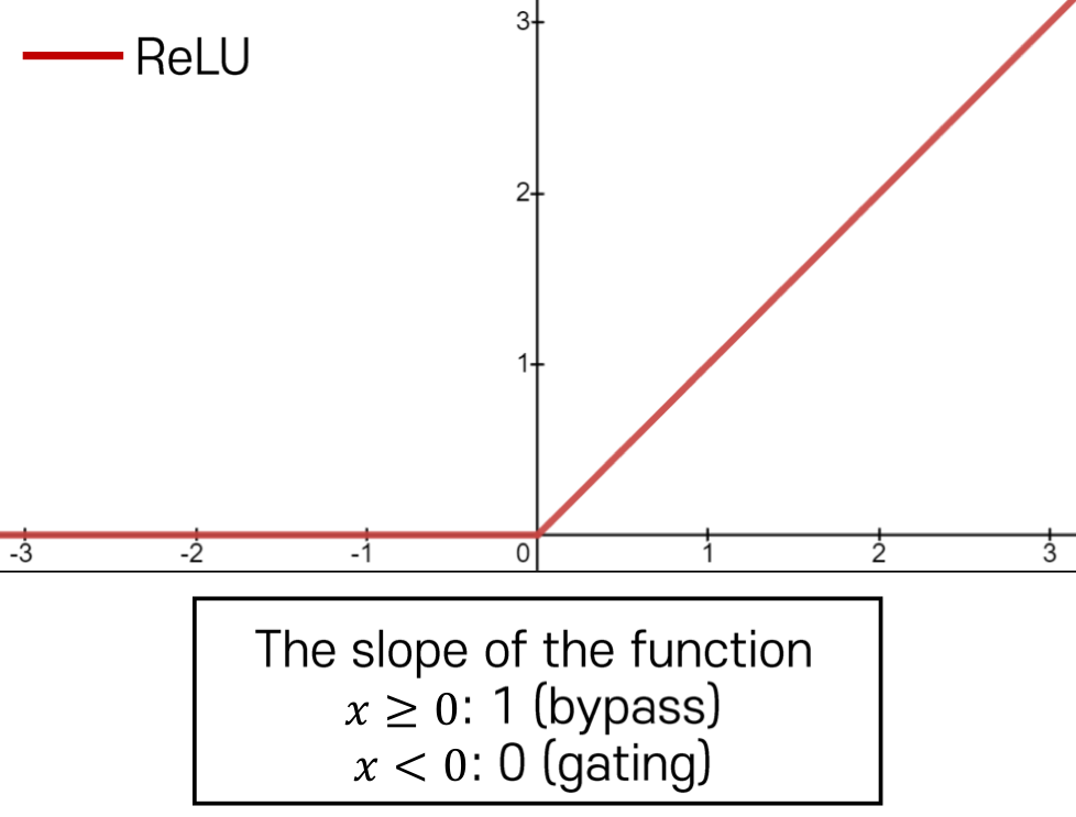
ReLU (Rectified Linear Unit)

• $f(x) = max(0,x)$
  Strength
• Does not saturate (in + region)
• Very computationally efficient
• Converge much faster than sigmoid/tanh

Weakness

• Not zeor-centered output
• Gradient is completely zero for $x < 0$

Batch Normalization

특정 활성함수를 썼을 때, 학습을 용이하게 하는 추가적인 특별한 형태의 뉴런 혹은 layer를 생각을 할 수가 있고, 그게 batch normalization이라는 layer이다.

• Saturated gradients when random initialization is done
• The parameters are not updated → Hard to optimize (in red region)

  Tanh activation
  데이터를 원하는 범위로 나눌 수 있으면 gradient vanishing 문제없이 학습이 용이하게 잘 될것
  → 기본적인 batch normalization 아이디어

Definition of Batch Normalization

"You want unit Gaussian activations? just make them so."

• We consider a batch of activations at some layer to make each dimension unit Gaussian

1. Compute the empirical mean $E[x^{(k)}]$ and variance $Var[x^{(k)}]$ independently for each dimension $k$
2. Normalize

This is a vanilla differentiable function

Batch Normalization Process

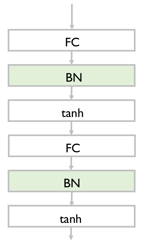
Usually inserted after fully-connected or convolutional layers, and before nonlinearity
→ 활성 함수 전에 추가하는 것이 일반적
Problem:
Do we necessarily want a unit Gaussian input to a tanh layer?

→ fully-connected layer를 통과를 시켜서 만들어진 출력 값들이 고유한 평균과 분산을 가지고 있고 그런 평균과 분산 자체도 우리 data item 그리고 우리 neural network가 학습해야 하는 중요한 정보를 담고 있는 경우에는 주어진 나름의 평균과 분산을 다 무시하고 평균, 분산 값을 무조건 0과 1로 만들어주는 변화는 어떤 의미에서는 neural network가 잘 추출한 정보를 잃어버리게 만드는 과정일 수 있다.