Machine Learning with PyTorch and Scikit-Learn_chapter6

Chapter6

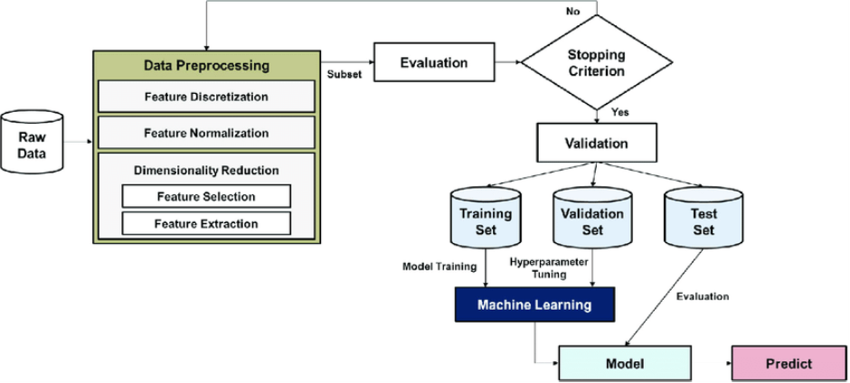
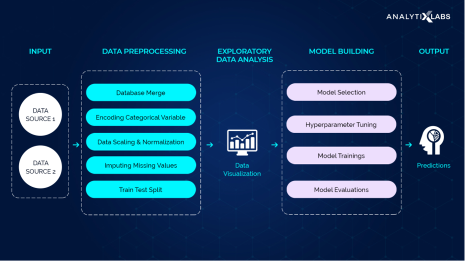
• Data preprocessing in the machine learning process

https://www.researchgate.net/figure/Data-preprocessing-in-the-machine-learning-process_fig4_342536324
https://www.analytixlabs.co.in/blog/data-preprocessing-in-machine-learning/

1. Pipeline

• The purpose of the pipeline is to assemble several steps that can be cross-validated together while setting different parameters. For this, it enables setting parameters of the various steps using their names and the parameter name separated by a '__', as in the example below. A step’s estimator may be replaced entirely by setting the parameter with its name to another estimator, or a transformer removed by setting it to 'passthrough' or None.
• Pipeline is a powerful tool to standardize your operations and chain them in sequence, make unions and fine-tune parameters.
• sklearn의 Pipeline class는 전처리, 모델 생성 및 학습 등을 포함하는 ML process를 한 번에 처리할 수 있게 해줌.

sklearn의 Pipeline class는 연속된 변환 단계를 순차적으로 처리하도록 돕는 tool로, 분류(또는 예측)을 위한 새로운 수학적 algorithm이 아님.

• Pipeline class는 transformer과 estimator를 감싼 일종의 Wrapper
  • Estimator(추정기): data set을 기반으로 일련의 모델 parameter들을 추정하는 객체.
  • Transformer(변환기): data set을 변환하는 estimator.

Sklearn_pipeline의 장점

• With Pipelines, your code is easier to read and understand. Hence less error-prone.
• You don’t have to call fit() and transform() methods for every transformers you write. You only have to call fit() and transform() once on the final Pipeline object.
• Pipelines help avoid leaking the test data into the trained model during cross-validation (Refer to this article to see how it helps)

### Pipeline 사용법
# 1. data set load

import pandas as pd

df = pd.read_csv('https://archive.ics.uci.edu/ml/'
                 'machine-learning-databases'
                 '/breast-cancer-wisconsin/wdbc.data', header=None)
df.head(20)


# 2. label encode

from sklearn.preprocessing import LabelEncoder

X = df.loc[:, 2:].values
y = df.loc[:, 1].values
le = LabelEncoder()
y = le.fit_transform(y)
le.classes_

le.transform(['M', 'B'])


# 3. split data set(train & test)

from sklearn.model_selection import train_test_split

X_train, X_test, y_train, y_test = \
    train_test_split(X, y, 
                     test_size=0.20,
                     stratify=y,
                     random_state=1)

# 4. create pipeline  *** main

from sklearn.preprocessing import StandardScaler
from sklearn.decomposition import PCA
from sklearn.linear_model import LogisticRegression
from sklearn.pipeline import make_pipeline

pipe_lr = make_pipeline(StandardScaler(),
                        PCA(n_components=2),
                        LogisticRegression(random_state=1))

pipe_lr.fit(X_train, y_train)
y_pred = pipe_lr.predict(X_test)
print('test accuracy: %.3f' % pipe_lr.score(X_test, y_test))

함수 설명:

1) make_pipeline(): sklearn transformers와 sklearn estimator를 연결.

• sklearn transformers: 입력에 대해 fit method와 transform method를 지원하는 객체.
• sklearn estimator: fit method와 predict method를 구현.

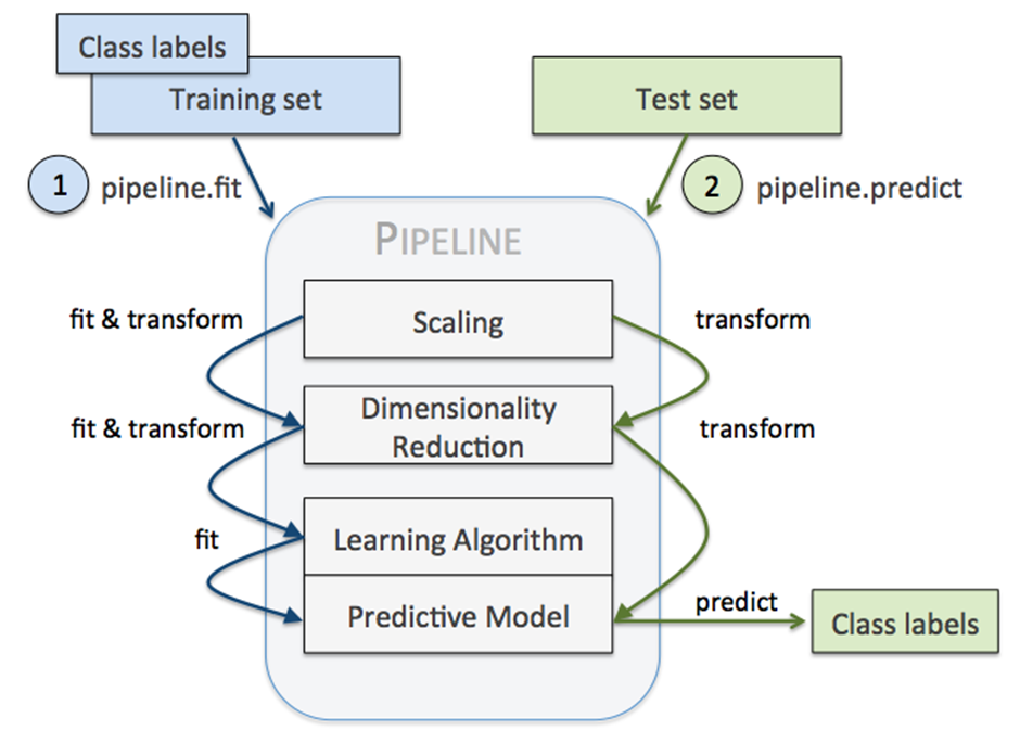
2) pipeline.fit(): 순차적으로 각 변환기의 fit_transform()이 실행되고, 각 단계의 output을 그 다음 단계의 input으로 전달. 가장 마지막 단계에서는 fit() method만 호출.

3) pipeline.predict(): 매개변수로 전달된 데이터가 각 단계의 transform() method를 통과. 가장 마지막 단계에서는 변환된 데이터에 대한 예측 값 return.

https://scikit-learn.org/stable/modules/generated/sklearn.pipeline.Pipeline.html
https://medium.com/@mannem16/a-simple-example-of-pipeline-in-ml-and-why-do-you-need-to-learn-it-6736795df72a
https://pythonsimplified.com/what-is-a-scikit-learn-pipeline/
https://dnai-deny.tistory.com/21
https://mindsee-ai.tistory.com/61
https://gils-lab.tistory.com/70

Pipeline 사용/미사용 비교

https://study2give.tistory.com/entry/%EB%A8%B8%EC%8B%A0%EB%9F%AC%EB%8B%9D-%ED%8C%8C%EC%9D%B4%ED%94%84%EB%9D%BC%EC%9D%B8Pipeline

2. 평가지표

Evaluation Metric은 일반적으로 모델이 Classification이냐 Regression이냐에 따라 다름.

• Regression: MAE , MSE, R^2
• Classification: Accuracy, Precision, Recall, F1 Score, ROC, AUC

2.1. Confusion Matrix

구축한 모델(Classifier)의 예측 결과가 얼마나 confusion한지 보여주는 지표.

• TP, TN, FP, FN 값들을 통해 모델의 성능을 측정할 수 있는 지표들을 알 수 있음(Accuracy, Precision, Recall).

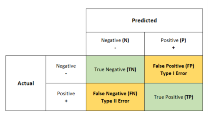
• True Positives (TP): when the actual value is Positive and predicted is also Positive.
• True negatives (TN): when the actual value is Negative and prediction is also Negative.
• False positives (FP): When the actual is negative but prediction is Positive. Also known as the Type 1 error
• False negatives (FN): When the actual is Positive but the prediction is Negative. Also known as the Type 2 error

Type 1 error 와 Type 2 error 예시) 귀무가설: 메일은 스팸이 아니다’

Type 1 error: 스팸이 아닌 메일이 스팸 박스로 보내진 경우(즉, 잘못된 인정)

Type 2 error: 스팸이 맞는 메일이 스팸 박스로 보내지지 않은 경우(즉, 잘못된 부정)

https://towardsdatascience.com/clarifying-type-i-and-type-ii-errors-in-hypothesis-testing-1a4e6a5ba616

2.2. 구축한 모델(Classifier)이 적합한지 측정할 수 있는 지표

Accuracy(정확도)

전체 문제 중, 정답을 맞춘 비율.

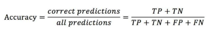
정확도만으로는 모델의 성능을 정확하게 판단하기 어려움.

• 왜냐하면, 문제 9개의 답이 1이고 문제 1개의 답이 0인 경우(총 10문제), 모든 문제의 정답이 1이라고 예측하는 모델을 구축하였더라도(잘못된 모델) 그 모델의 accuracy가 90%.
• Accuracy is not a good metric to use when you have class imbalance
  참고) ERR(예측 오차) = 1 – ACC(정확도)

Precision(정밀도)

예측을 Positive로 한 대상 중, 예측 값과 실제 값이 Positive로 일치한 데이터의 비율

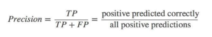
• FP가 낮을수록, 점수가 커짐(Type 1 error를 낮추는데 초점).

Recall(재현율, also known as Sensitivity or TPR(True Positive Rate))

실제 값이 Positive인 대상 중, 예측 값과 실제 값이 Positive로 일치한 데이터의 비율.

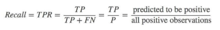
• FN이 낮을수록, 점수가 커짐(Type 2 error를 낮추는데 초점).

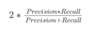
F-1 score

F1 score sort of maintains a balance between the precision and recall for your classifier.

• Precision과 recall 모두 활용하여 계산(precision과 recall을 조합하여 하나의 값을 산출).
  

https://medium.com/analytics-vidhya/what-is-a-confusion-matrix-d1c0f8feda5

ROC curve (Receiver Operating Characteristic curve)

• ROC는 Sensitivity와 Specificity의 관계를 curve로 표현한 것(정확하게는 TPR(x축)과 FPR(1 - Specificity)(y축)을 활용하여 그래프를 그림).
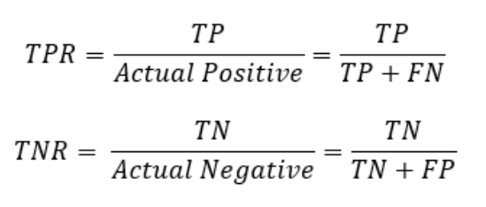
• Sensitivity: TPR(True Positive Rate; recall)
• Specificity: TNR(True Negative Rate) or 1 - FPR(False Positive Rate)
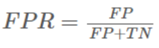
  - FPR(False Positive Rate)는 정답이 1인데 0이라고 말한 비율.

---

계산 예)
TP: 3 TN: 2
FP: 2 FN: 1

sensitivity = TP / (TP + FN) = 3 / (3 + 1) = 3/4 = 0.75
specificity = TN / (TN + FP) = 2 / (2 + 2) = 2/4 = 0.5
FPR = FP / (FP + TN) = 0.5

---

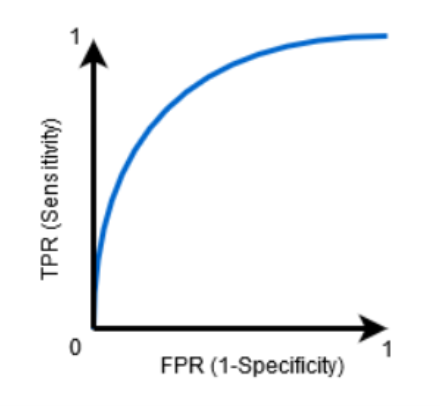
• X축으로 Specificity가 아닌 1 – specificity를 활용하는 이유: 우상향 그래프가 그래프를 읽이 수월하기 때문.

---

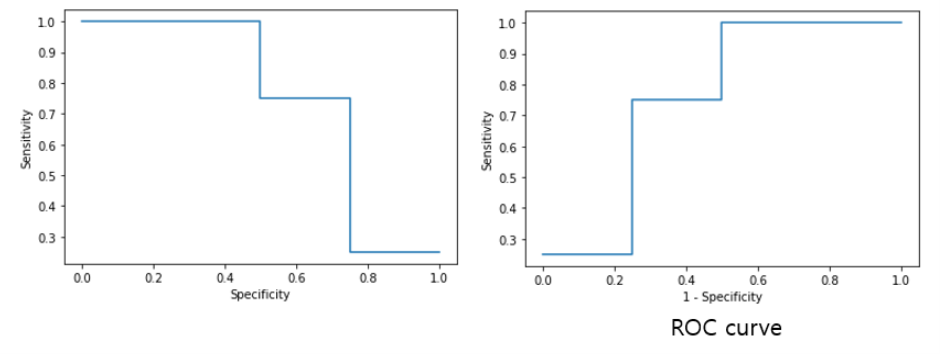
참고) TPR 과 FPR의 관계.
True: 잘된 답을 찾았음을 의미.
False: 잘못된 답을 찾았음을 의미.
Positive: 질문에 대한 답을 YES라고 했음을 의미.

• True positive: 실제 스팸 메일일 때, 스팸 메일이 맞다고 판단한 것.
• False positive: 실제 스팸 메일이 아닐 때, 스팸 메일이 맞다고 판단한 것.
  A라는 스팸 메일 분류기가 모든 메일에 대해 스팸 메일이라고 판단한다면, TPR과 FPR이 모두 올라갈 것(왜? 무조건 다 스팸이라고 하니까).
• 즉, TPR과 FPR은 정비례 관계.
• 그런데 Sensitivity와 Specificity는 반비례 관계(당연히 Specificity가 1-FPR이니까).

---

ROC curve의 필요성
https://towardsdatascience.com/understanding-the-roc-curve-and-auc-dd4f9a192ecb

AUC (Area Under the Curve)

ROC curve 곡선 밑부분, 1에 가까울수록 성능이 좋다고 판단.

• ROC curve의 밑부분인 AUC 값을 통해, classification 모델의 성능을 판단.

https://www.analyticsvidhya.com/blog/2020/06/auc-roc-curve-machine-learning/
https://derangedphysiology.com/main/cicm-primary-exam/required-reading/research-methods-and-statistics/Chapter%203.0.5/receiver-operating-characteristic-roc-curve

추가)
https://angeloyeo.github.io/2020/08/05/ROC.html
https://funmi.tistory.com/6
https://www.kdnuggets.com/2022/08/type-type-ii-errors-difference.html

3. Cross-validation(교차 검증)

• 통계적 평가 방법
• 주어진 data set을 학습한 algorithm이 얼마나 잘 일반화되었는지 평가할 때 사용.
• 모델 학습시 데이터를 훈련용(train)과 검증용(test)으로 교차하여 선택하는 방법.

=> 교차 검증의 목적: overfitting을 피하면서 parameter를 튜닝하고 general한 모델을 만들고 더 신뢰성 있는 모델 평가를 하기 위해.

=> Holdout cross-validation과 K-fold cross-validation은 대표적인 cross-validation 방법.

Cross-validation을 이해하기에 앞서 training set / validation set / test set에 대해 알아야 함.

• Train Set: Used to train the model.
• Validation Set: Used to tune the parameters like K in K-NN or the number of hidden layers in a Neural Network(Used to optimize model parameters).
• Test Set: Used to asses the performance of a fully-trained model.

train set과 test set으로만 data를 분리하면(validation set 없이), 모델을 검증하기 위해 test set만 사용하게 됨.

• 여기서, 고정된 test set으로 ' 모델의 성능을 확인 -> parameter 수정 -> 모델의 성능을 확인 ' 과정을 반복하면 최종 모델은 test set에 over-fitting 되어 unseen data(실제 예측하고자 하는 data)에 대한 예측력이 떨어질 수 있음. 이를 예방하고자 활용되는 것이 validation set.

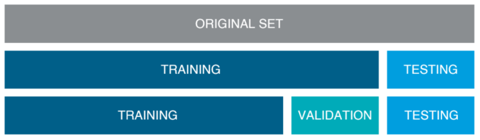
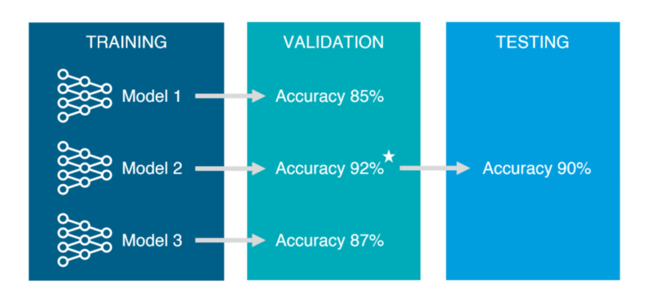
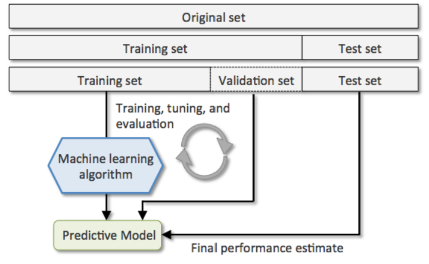
=> 즉, training set으로 모델을 만들고, validation set으로 parameter을 튜닝하고 사용할 모델을 선택, test set으로 선택한 모델을 최종적으로 평가.

• train set 중 일부를 validation set으로 활용하기 때문에 data의 절대량이 적을 때는 오히려 학습시킬 데이터가 줄어들게 되어 효용을 기대할 수 없게 될 수 있음.

https://modern-manual.tistory.com/19
https://www.statology.org/validation-set-vs-test-set/
https://towardsdatascience.com/train-validation-and-test-sets-72cb40cba9e7
https://wkddmswh99.tistory.com/m/10
https://for-my-wealthy-life.tistory.com/m/19

3.1. Holdout cross-validation

가장 기초적인 방법으로 전체 data set을 설정한 비율에 맞춰 아래와 같이 나누는 것.
1) train set : test set
2) train set : validation set : test set

3.2. K-fold cross-validation

K개의 fold를 만들어서 진행하는 cross-validation(즉, k개의 data set을 구성하고 각각 학습).

• K는 사용자 지정 hyper parameter(good standard value for k in k-fold cross-validation is 10, data set의 크기가 클 때에는 5를 사용하는 것을 추천).
• Randomly split the training data set into k folds(중복 불허).
• K-1개의 fold로 model training(training set), 1개의 fold로 model test(test set). 이 과정으로 k번 반복하여 k개의 model과 k개의 performance estimates를 얻음.
• k개의 결과에 대한 평균 값을 산출한 뒤, 최종 성능을 구함.
  - 고정된 test set으로 구한 결과값이 아니므로, hold out 방식 보다 결과값을 일반화할 수 있음.

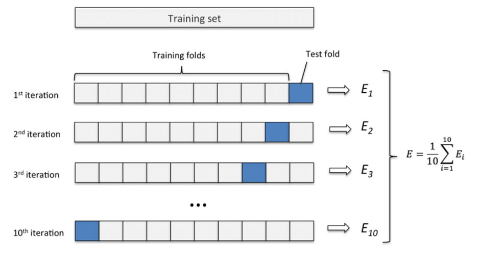
• k-fold cross validation (k=10)

The algorithm of the k-Fold technique
1) Pick a number of folds – k. Usually, k is 5 or 10 but you can choose any number which is less than the dataset’s length.
2) Split the dataset into k equal (if possible) parts (they are called folds)
3) Choose k – 1 folds as the training set. The remaining fold will be the test set
4) Train the model on the training set. On each iteration of cross-validation, you must train a new model independently of the model trained on the previous iteration
5) Validate on the test set
6) Save the result of the validation
7) Repeat steps 3 – 6 k times. Each time use the remaining  fold as the test set. In the end, you should have validated the model on every fold that you have.
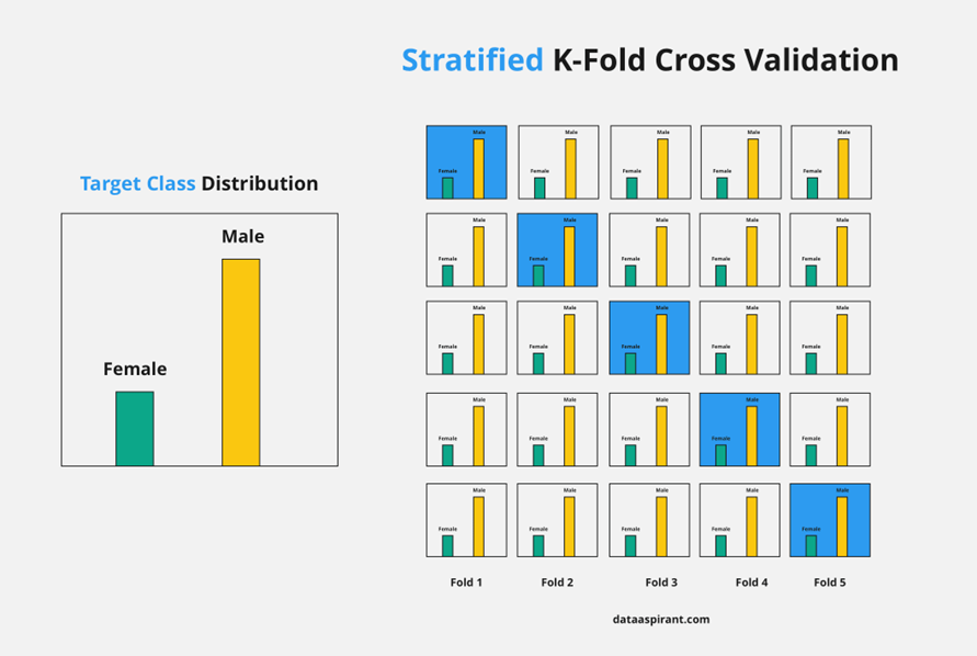
8) To get the final score average the results that you got on step 6.

3.3. Stratified K-fold Cross Validation

K-fold Cross Validation의 변형된 방식으로 data가 편항되어 있는 경우(즉, imbalanced data의 경우) 사용됨.

• imbalanced data의 경우, n번째 fold의 test set에 특정 class가 몰리는 상황이 발생할 수 있음(예, 극단적인 예로 training set과 test set을 8:2로 나누는 상황에, 데이터의 분포가 y = 1 : y = 0 이 8:2 이라면, training set에 y = 1이 8, test set에 y = 0이 2 할당되는 경우)
• Stratified K-fold Cross Validation은 전체 data set의 class(의 비율)를 고려하여, set을 구성함.

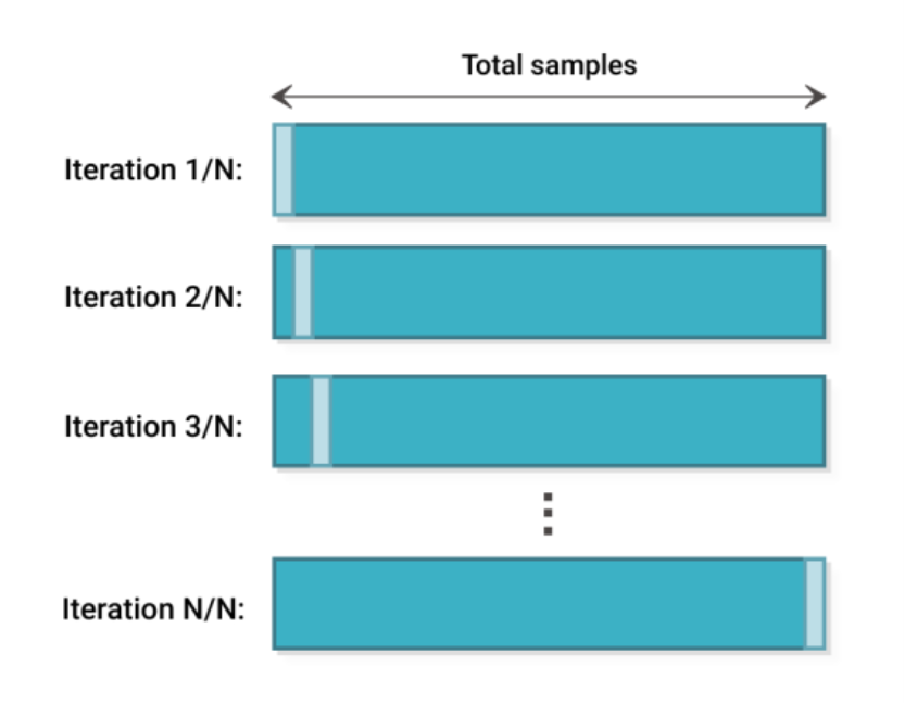
3.4. Leave One Out Cross Validation(LOOCV)

Leave-one-out сross-validation (LOOCV) is an extreme case of k-Fold CV. Imagine if k is equal to n where n is the number of samples in the dataset. Such k-Fold case is equivalent to Leave-one-out technique.

Recommended approach for working with vert small data sets.

https://neptune.ai/blog/cross-validation-in-machine-learning-how-to-do-it-right
https://blog.naver.com/winddori2002/221850530979

4. Grid search

• model의 성능 향상에 최적화된 hyper parameter를 찾는 방법.
• hyper parameter의 후보군이 될 수 있는 값들을 list 형태로 넣은 뒤, 모든 경우에 대한 model을 만들고 성능을 평가함(가장 좋은 하나의 경우를 찾음).
• 사용자가 원하는 hyper parameter 후보군을 비교 분석할 수 있음(후보군을 직접 넣기 때문에).

---

parameter와 hyper parameter의 차이.

parameter: A model parameter is a configuration variable that is internal to the model and whose value can be estimated from data.

• They are estimated or learned from data.
• They are often not set manually by the practitioner.
  예) 랜덤 포레스트 모델에서 weight 설정.

hyper parameter: A model hyperparameter is a configuration that is external to the model and whose value cannot be estimated from data.

• They are often specified by the practitioner.
  예) 랜덤 포레스트 모델에서 tree의 depth 설정.

=> 사용자가 직접 설정하면 하이퍼 파라미터, 모델 혹은 데이터에 의해 결정되면 파라미터

https://machinelearningmastery.com/difference-between-a-parameter-and-a-hyperparameter/

---

Grid search의 경우 hyper parameter의 후보군이 될 수 있는 값들을 바탕으로 경우의 수를 전부 따지기 때문에 후보군이 많을 수록, 시간이 오래 걸림. 속도면에서 장점이 있는 Randomized search 방법이 있음.

5. Randomized search

• Grid search와 유사한 방식으로 작동, 최적화된 hyper parameter를 찾는 방법.
• hyper parameter의 후보가 될 수 있는 값들의 range와 반복 추출할 횟수(n_iter)를 지정한 뒤, 매 횟수(n_iter 만큼) 마다 random한 hyper parameter를 뽑아 그 값을 모델에 대입하여 성능을 평가.
• Grid search에서 후보군이 되지 않은 hyper parameter가 모델에 대입될 수 있다.

n_iter: Number of parameter settings that are sampled

https://cori.tistory.com/167
http://www.jmlr.org/papers/volume13/bergstra12a/bergstra12a.pdf

---

참고)
Halving Grid seach
https://bobrupakroy.medium.com/halving-gridsearch-736b13898327

Bayesian Optimization
https://shinminyong.tistory.com/37
https://data-scientist-brian-kim.tistory.com/88

---

6. nested cross-validation

• 기존의 cross-validation을 중첩한 방법.
• Outer loop와 Inner loop로 구성되어 있음.
• Outer k-fold cross-validation loop which is used to split the data into training and test folds.
• Inner k-fold cross-validation loop hat is used to select the most optimal model using the training and validation fold.

https://vitalflux.com/python-nested-cross-validation-algorithm-selection/

• 5×2 cross validation

Outer loop 각각의 fold는 train set과 test set으로 구성되어 있음. 여기서, train set에 Inner loop가 작동함. Inner loop는 train set(Outer loop에 있는)을 train set’과 validation set으로 분리한 뒤, 평가 과정을 통해 parameter를 튜닝. 그 후 Optimal한 parameter를 찾고 이 optimal한 parameter을 통해 outer loop의 test set을 평가. 이 과정을 k번 반복(k-fold).

=> 요약하면, inner loop는 각 fold의 parameter를 튜닝하고 outer loop는 test set에 대한 평가.

=> nested cross-validation은 각 fold에 맞는 optimal한 parameter가 적용된 여러 test set의 평가 정보를 바탕으로 보다 일반화된 model을 구하고자 함.

7. Dealing with class imbalance

class가 imbalance한 데이터를 그대로 ML model에 적용하면 안됨(예, y=1이 전체 데이터의 90%, y=0가 10%인 불균형한 데이터가 주어졌을 때, 항상 y=1로 분류하는 model의 정확도는 90%).

Class imbalance 해소 방법.

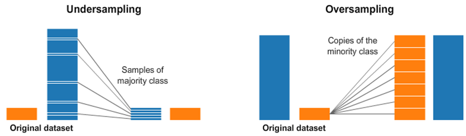
1) downsampling the majority class

• Under sampling
  majority class의 data 일부를 버리는 방식으로 class간 균형을 맞추는 방법.
  잠재적으로 가치가 높은 data를 잃게 될 위험이 있음(data의 소실).

2) upsampling the minority class

• Over Sampling
  minority class의 data를 복원 추출해 class간 균형을 맞추는 방법.
  동일한 data를 복원 추출하기 때문에 over-fitting 위험도 증가.

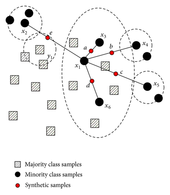
3) the generation of symthetic training examples.

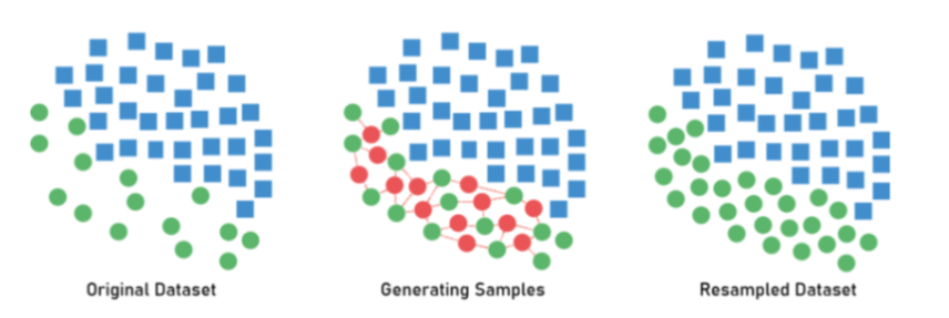
• Algorithm Over Sampling: Synthetic Minority Over-sampling Technique(SMOTE)
  minority class에서 각각의 sample들의 k-nearest neighbors를 찾고, 다음으로 이웃들 사이에 선을 그어 무작위 점(data point)를 생성.
  - 두 data point(sample) 사이에서 각각의 특성을 반영한 data point가 생성.

https://dining-developer.tistory.com/27