주성분 분석(PCA)
주성분 분석(PCA)은 고차원 데이터에서 차원을 축소하거나 데이터의 주요 패턴을 찾는데 사용된는 알고리즘이다. 고차원 데이터는 복잡하고 *노이즈가 많아 분석이 어려울 수 있으므로, PCA를 통해 데이터의 핵심 정보를 추출하거나 차원을 낮출 수 있다.
1. 주요 개념
1) 차원(Dimension)
데이터에서 하나의 특성을 의미한다. 예를 들어, 이미지 데이터는 픽셀 값으로 구성된 다차원 데이터이다.
2) 차원 축소(Dimension Reduction)
데이터의 차원을 줄여서 분석을 쉽게 하거나 노이즈를 줄이는 과정이다
3) 분산(Variance)
데이터가 얼마나 다양하게 분포되어 있는지를 나타낸다. 분산이 크면 그 방향이 데이터의 변동성이 크다는 의미이다.
4) 주성분(Principal Components)
PCA에서 분산이 가장 큰 방향을 찾은 결과물이다. 각 주성분은 데이터의 주요 패턴을 나타내며, 고유벡터(eigenvectors)로 표현된다.
💡 노이즈
유용한 정보와 무관하거나 방해가 되는 데이터를 의미한다.
노이즈는 데이터의 정확성, 품질 또는 분석 결과에 영향을 미칠 수 있으며, 노이즈가 많을수록 모델의 성능이 떨어지거나 예측이 부정확해질 수 있다.
2. PCA 예제
import numpy as np
fruits = np.load('fruits_300.npy')
fruits_2d = fruits.reshape(-1, 100*100)

# 주성분 분석 알고리즘
from sklearn.decomposition import PCA
pca = PCA(n_components=50) #주성분 개수 50
pca.fit(fruits_2d)

# 배열 크기
print(pca.components_.shape)
#출력 (50, 10000)

import matplotlib.pyplot as plt
def draw_fruits(arr, ratio=1):
  n = len(arr)
  rows = int(np.ceil(n/10)) # 행의 개수
  cols = n if rows < 2 else 10
  fig, axs = plt.subplots(rows, cols, figsize=(cols*ratio, rows*ratio), squeeze=False)
  for i in range(rows):
    for j in range(cols):
      if i*10 + j < n:
        axs[i, j].imshow(arr[i*10 + j], cmap='gray_r')
      axs[i, j].axis('off')
  plt.show()

# 주성분 이미지 출력
draw_fruits(pca.components_.reshape(-1, 100, 100))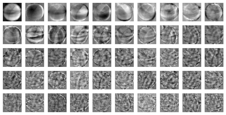
3. PCA를 사용한 차원 축소
print(fruits_2d.shape)
# (300, 10000)
# 특성의 개수를 줄임
fruits_pca = pca.transform(fruits_2d)
print(fruits_pca.shape)
# #출력 (300, 50)

# 특성 복원
fruits_inverse = pca.inverse_transform(fruits_pca)
print(fruits_inverse.shape)
#출력 (300, 10000)fruits_2d를 PCA로 변환하면, 원본 데이터에서 가장 중요한 50개의 주성분으로 차원이 축소된다.- 차원을 축소한 후,
pca.invers_transform을 통해 원래 데이터로 재구성할 수 있다.
4. 설명된 분산(Explained Variance)
print(np.sum(pca.explained_variance_ratio_))
#출력 0.9215484019814356

plt.plot(pca.explained_variance_ratio_)
plt.show()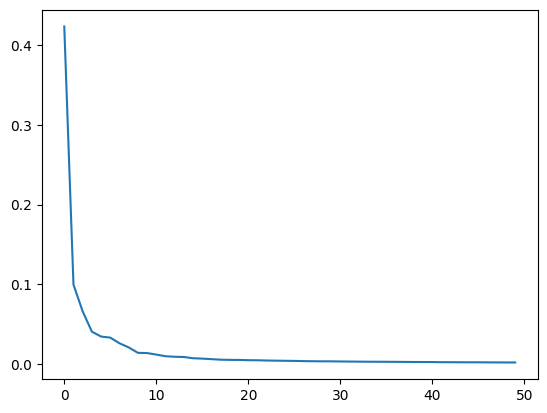
pca.exlarined_variance_ratio_는 각 주성분이 전체 분산에서 얼마나 많은 부분을 설명하는지 나타낸다.- 주성분을 선택할 때, 설명된 분산 비율을 활용하여 최적의 주성분 개수를 결정할 수 있다.
5. PCA와 다른 알고리즘의 조합
# 로지스틱 회귀 모델 사용
from sklearn.linear_model import LogisticRegression
lr = LogisticRegression()

# 타깃 데이터
target = np.array([0] * 100 + [1] * 100 + [2] * 100)

from sklearn.model_selection import cross_validate
#교차 검증
#축소하지 않은 데이터 학습 점수와 학습 시간
scores = cross_validate(lr, fruits_2d, target)
print(np.mean(scores['test_score']))
#출력 0.9966666666666667
print(np.mean(scores['fit_time']))
#출력 2.2455021381378173

#축소된 데이터 학습 점수와 학습 시간
scores = cross_validate(lr, fruits_pca, target)
print(np.mean(scores['test_score']))
#출력 1.0
print(np.mean(scores['fit_time']))
#출력 0.035051822662353516

#설명된 분산 50%에 해당하는 주성분
pca = PCA(n_components=0.5)
pca.fit(fruits_2d)

print(pca.n_components_)
#출력 2 #2개의 특성으로 분산의 50% 표현

fruits_pca = pca.transform(fruits_2d)
print(fruits_pca.shape)
#출력 (300, 2)

#2개의 특성으로 축소된 데이터 확인
scores = cross_validate(lr, fruits_pca, target)
print(np.mean(scores['test_score']))
#출력 0.9933333333333334
print(np.mean(scores['fit_time']))
#출력 0.03991680145263672

#k-평균 알고리즘으로 클러스터 확인
from sklearn.cluster import KMeans
km = KMeans(n_clusters=3, random_state=42)
km.fit(fruits_pca)
print(np.unique(km.labels_, return_counts=True))
#출력 (array([0, 1, 2], dtype=int32), array([110,  99,  91]))

# 삼전도
for label in range(0, 3):
  data = fruits_pca[km.labels_ == label]
  plt.scatter(data[:,0], data[:,1])
plt.legend(['apple', 'banana', 'pineapple'])
plt.show()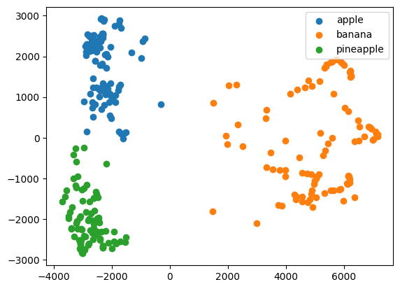
- 로지스틱 회귀 모델을 사용하여, PCA를 적용하지 않은 데이터와 적용한 데이터의 학습 시간을 비교할 수 있다. PCA를 사용하면 학습 시간이 크게 단축된다.
- PCA를 통해 50% 이상의 분산을 설명하는 주성분을 찾을 수 있으며, 이를 사용해 데이터의 차원을 줄이고도 좋은 모델 선능을 유지할 수 있다.
- KMeans와 같은 클러스터링 알고리즘과 결합하여, 데이터의 주요 클러스터를 식별할 수 있다.