[Linear Viscoelasticity] 03. Static Test

jmt·2024년 2월 22일

creep complaince creep test linearity check relaxation modulus static test stress relaxation test 고분자 선형점탄성 유변학

선형점탄성(Linear Viscoelasticity)

목록 보기

4/7

Static Test

앞에서 선형 점탄성은 시스템의 선형성을 이용하여, Boltzmann Superposition Principle(BSP) 활용해 strain과 stress를 system의 response function, 즉 material function에 해당하는 Relaxation Modulus, $G(t)$ 와 Creep Compliance, $J(t)$ 로 표현해보았다. 그렇다면 실제 고분자 물질을 가지고 유변 물성을 알아보기 위해 실험을 해보자. 선형 점탄성 거동을 알아보기 위한 실험은 크게 2가지가 있다. Static Test와 Dynamic Test이다. static test에 해당되는 실험은 Stress Relaxation Test와 Creep Test가 있는데, static 이라 부르는 이유는 system에 가하는 stimulation이 $t>0$ 에서 상수로 주어지기 때문이다.

Stress Relaxation Test

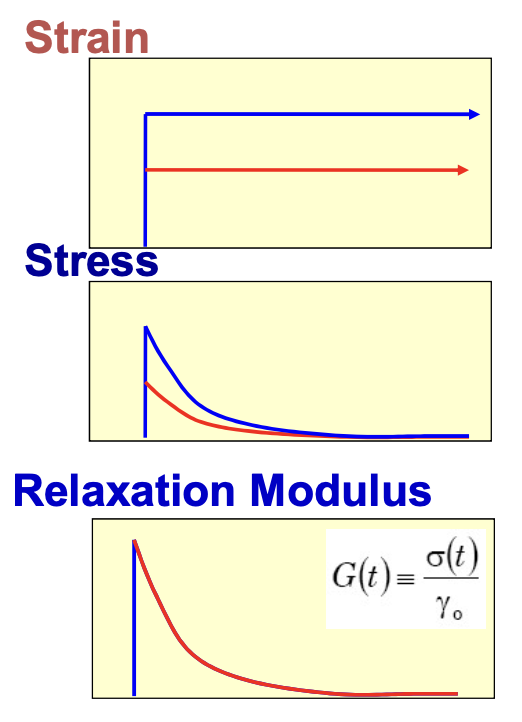
stress relaxation test는 strain, $\gamma$ 을 input으로 주고 stress, $\sigma$ 를 측정하는 실험이다. 앞에서 배웠던 내용을 떠올려보면 다음과 같은 유도가 가능하다.

\begin{aligned} \sigma(t) &= F[\gamma(t)]\\ &= F[\gamma_0\Theta(t)]\\ &= \gamma_0 F[\Theta(t)]\\ G(t) &= \frac{\sigma(t)}{\gamma_0}=F[\Theta(t)]\\ \end{aligned}

위에 그림을 보면 알 수 있듯이 $G(t) \ge 0$ 이고 $\frac{dG}{dt}\le 0$ 임을 알 수 있다.

Linearity Check

선형 응답 조건을 만족한다면 $G(t)$ 는 겹치게 된다. $n$ 개의 strain amplitude를 $\gamma_k$ 라고 정의하고, 측정한 stress를 $\sigma_k(t)$ 라고 하자. $\gamma_1 < \gamma_2 < \cdots < \gamma_n$ 일 때, $G_k(t)=\sigma_k(t) / r_k$ 이므로, $G_1 = G_2 = \cdots = G_n$ 이여야 한다. 그렇다면 우리는 $n$ 개의 strain에 따른 $n$ 개의 relaxation modulus를 구할 수 있는데, 선형성을 만족하는 $\gamma_{max}$ 를 찾을 수 있다. 아래 plot 중 왼쪽은 stress relaxation test에서 다른 $\gamma_0$ 에 대해서 t에 따른 stress를 그린 것이고, 오른쪽은 구한 relaxation modulus를 t에 대해 그린 것이다.

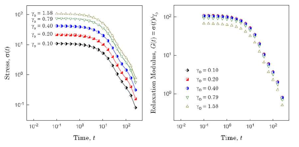
대략 $\gamma_0 \le 0.40$ 까지는 잘 맞지만, constant strain이 그보다 커지는 경우 선형성을 만족하지 못한다는 것을 알 수 있다.

왜 $\gamma_{max}$ 를 구해야할까?

stress relaxation test에서 보이는 선형 점탄성 거동은 strain이 작은 경우 계가 평형에 가깝기 때문에 나타나는 현상이다. 점탄성은 앞서 배웠듯, 분자열운동에 의한 완화가 응력완화로 관찰되는 현상이기 때문이다. 즉 constant strain에 의해 계가 평형상태에서 벗어난 비평형상태가 되고, 분자의 열운동에 의해 다시 평형상태로 되돌아온다. 이것이 stress relaxation test에서 응력의 감쇠로 관찰되는 것이다. 즉, 주어진 constant strain이 작다면 평형상태에서 벗어난 비평형상태에서의 계는 평형상태의 근방에 있기 때문에 계에 선형응답성이 존재하게 된다. 그렇다면 굳이 $\gamma_{max}$ 를 구하지 않고 아주 작은 constant strain을 사용하면 되지 않을까?

stress relaxation test에서 사용하는 strain-controlled rheometer는 output인 stress를 측정하기 위해 돌림힘 센서(torque sensor)를 이용한다. 돌림힘을 통해 응력을 구하는 공식이 존재하기 때문이다. 그런데 이 돌림힘 센서는 작은 constant strain으로 인해 발생하는 stress signal를 잘 인식하지 못하게 된다. 그렇기 때문에 실험 결과에 오차가 작용하게 되어 신뢰할 수 없는 결과를 도출해낼 수 있다.

Formal Expression of $G(t)$

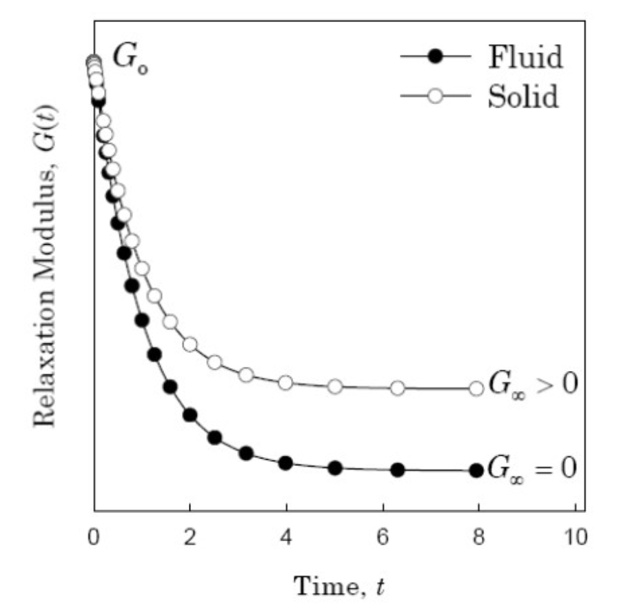
위 plot은 stress relaxation test로 t에 따른 Relaxation Modulus, $G(t)$ 를 그린 것이다. 고체의 경우 0에 수렴하게 되고, 액체의 경우에는 0보다 큰 상수값에 수렴하게 된다는 것을 알 수 있다. relaxation modulus는 시간에 따라 감쇠하는 것으로 보인다. 그러므로 모든 $t$ 에 대해

\frac{dG}{dt} \ge 0

임을 알 수 있다. 그리고 stress relaxation test에서 strain은 $\gamma(t) = \gamma_0\Theta(t)$ 로 정의하였기 때문에 stress는 다음과 같이 표현된다.

\begin{aligned} \sigma(t) &= F[\gamma(t)]\\ &= \gamma_0G(t) \end{aligned}

만약 임의의 시간에서 relaxation modulus가 증가한다면, 아주 작은 strain으로도 stress가 무한히 증가할 수 있기 때문에 일어날 수 없는 일이다. 그러므로 $G(t)$ 는

0\le G(t) \le G_{max}

이다. 0보다 커야하는 이유는 만약 $G(t)<0$ 이라면, strain에 대해 stress의 방향이 서로 반대가 되어야한다. 이는 현실적으로 불가능하다. 그럼 이제 우리는 $G(t)$ 를 다음과 같은 형태로 표현할 수 있다.

G(t) = [G_{\infin}+(G_0+G_{\infin})\phi(t)]\Theta(t)

where

\begin{aligned} \phi(t) \ge 0;\quad \phi(0)=1;\quad \lim_{t\rightarrow\infin} \phi(t)=0;\quad \frac{d\phi}{dt}\le0 \end{aligned}

그리고 $G_0>G_{\infin}>0$ 이고 고체의 경우에는 $G_{\infin}=0$ , 액체의 경우에는 $G_{\infin}>0$ 이다.

Creep Test

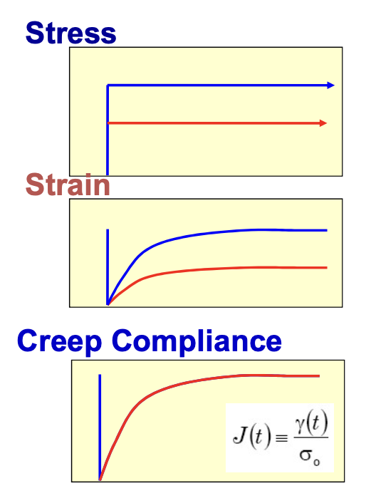
creep test는 stress를 input으로 strain을 output으로 측정하여 response function이자 material function인 Creep Compliance를 알아보는 실험이다. stress relaxation test와 동일하게 다음과 같은 유도를 따른다.

\begin{aligned} \gamma(t) &= F^{-1}[\sigma_0\Theta(t)]\\ &= \sigma_0 F^{-1}[\Theta(t)]\\ J(t) &= \frac{\gamma(t)}{\sigma_0}=F^{-1}[\Theta(t)] \end{aligned}

또한, 위의 실험 결과를 통해 $J(t)\ge 0$ 이고, $\frac{dJ}{dt} \ge 0$ 임을 알 수 있다.

Formal Expression of $J(t)$

BSP로 creep compliance를 구하였고, creep test로 나타나는 성질을 시간의 함수로 나타내보자.

\begin{aligned} J(t) = \begin{cases} [\frac{1}{G_0} + J_r \psi(t) + \frac{t}{\eta_0}]\Theta(t)\quad for\;fluid\\ [\frac{1}{G_0} + J_r \psi(t)]\Theta(t)\quad\quad\quad for\; solid \end{cases} \end{aligned}

where

\psi(0)=0;\quad \lim_{t\rightarrow\infin}\psi(t)=1;\quad \frac{d\psi}{dt}\ge 0

Laplace transform of $\gamma(t), \sigma(t)$

BSP로 $\gamma(t), \sigma(t)$ 를 합성곱(convolusion)의 형태로 나타낼 수 있었다.

\begin{aligned} \sigma(t) &= \int^t_{\infin} G(t-\tau)\frac{d\gamma}{d\tau}d\tau\\ \gamma(t) &= \int^t_{\infin} J(t-\tau)\frac{d\sigma}{d\tau}d\tau \end{aligned}

이를 라플라스 변환(Laplace Transform)하면 다음과 같다. 라플라스 변환을 $\mathfrak{L}[f(x)] \equiv \tilde f(s)$ 로 표현하도록 하자.

\begin{aligned} \tilde \sigma(s) &= \tilde G(s) \cdot \mathfrak{L} [\dot \gamma(t)]\\ &= \tilde G(s) \cdot \{s \tilde \gamma (s) - \gamma(0^-)\}\\ &= s\tilde G(s)\tilde\gamma(s)\\ \tilde \gamma(s) &= \tilde J(s) \cdot \mathfrak{L} [\dot \sigma(t)]\\ &= \tilde J(s) \cdot \{s \tilde \sigma(s) - \sigma(0^-)\}\\ &= s \tilde J(s)\tilde\sigma(s) \end{aligned}

최종적으로 $G(t)$ 와 $J(t)$ 의 관계는 다음과 같다.

s\tilde G(s) =\frac{1}{s \tilde J(s)}

steady-state compliance and zero-shear viscosity

앞에서 라플라스 변환을 응용하여 relaxation modulus와 creep compliance의 관계를 알아보았다. 이를 통해 고체일 때 다음이 성립함을 알 수 있다.

\frac{1}{G_{\infin}} = \frac{1}{G_0}+J_r

액체일 때는 creep compliance는 다음과 같은 거동을 보인다 할 수 있다.

J(t) = J^0_e+\frac{t}{\eta_0}\quad for\;large\;t

이제 steady-state compliance를 다음과 같이 정의하자.

J^0_e=\frac{1}{G_0}+J_r

또한 zero-shear viscosity는 다음과 같이 정의된다.

\eta_0 = G_0\int^{\infin}_0 \phi(t) dt

\eta_0 = \int^{\infin}_0 G(t)dt

jmt

고분자/컴공

이전 포스트

[Linear Viscoelasticity] 02. Boltzmann Superposition Principle (BSP)

다음 포스트

[Linear Viscoelasticity] 03. Static Test

선형점탄성(Linear Viscoelasticity)

Static Test