[Linear Viscoelasticity] 04. Dynamic Test

jmt·2024년 2월 22일

Fourier Transform dynamic moduli dynamic test loss modulus storage modulus terminal behavior 고분자 선형점탄성 유변학

선형점탄성(Linear Viscoelasticity)

목록 보기

5/7

Dynamic Test

static test에 해당되는 stress relaxation test와 creep test를 통해 relaxation modulus, $G(t)$ 와 creep compliance, $J(t)$ 를 구할 수 있었다. static test는 $t>0$ 에서 system에 가하는 stimulation을 unit-step function으로 준다. 실험에서 현실적으로 완벽한 unit-step function으로 구하기엔 어렵다. 하지만 우리는 sinusodial한 stimulation을 만들기는 쉽다. 즉, unit-step function이 아닌 sinusodial function을 system의 impulse function으로 가하는 실험을 dynamic test라고 한다.

Dynamic Moduli

strain을 $\gamma(t)=\gamma_0 \sin\omega t$ 로 두자. 여기서 $\gamma_0$ 는 strain amplitude이고, $\omega$ 는 주파수에 해당한다. 그럼 BSP에 의해 $\sigma(t)$ 는 다음과 같다.

\sigma(t) = \gamma_0 \omega \int^t_{-\infin} G(t-\tau)\cos\omega\tau d\tau

여기서 $\xi\equiv t-\tau$ 로 치환하여 다시 쓰면,

\sigma(t) = G^{\prime}\omega \gamma(t) + \eta^{\prime}\dot\gamma(t)

where $\dot\gamma(t) = d\gamma / dt$ , and

G^{\prime}(\omega) \equiv \omega \int^{\infin}_0 G(t)\sin\omega tdt;\quad \eta^{\prime} \equiv \int^{\infin}_0 G(t) \cos\omega t dt

만약, $G^{\prime}=0$ 이면, $\sigma(t)=\eta^{\prime}\dot\gamma(t)$ 가 되고 이 식은 viscous fluid의 구성방정식이 된다. 또한 $\eta^{\prime}=0$ 이면, $\sigma(t)=G^{\prime}(\omega)\gamma(t)$ 가 되고 이 식은 elastic solid가 된다. elastic solid는 에너지를 저장하고(탄성), viscous fluid는 역학적 에너지를 방출한다(점성). 그러므로 $G^{\prime}(\omega)$ 는 storage modulus, $G^{\prime\prime}(\omega)$ 은 loss modulus로 정의한다. $G^{\prime\prime}(\omega)$ 은 다음과 같이 정의할 수 있다.

G^{\prime\prime}(\omega) = \omega\eta^{\prime}(\omega) = \omega \int^{\infin}_0 G(t)\cos\omega t dt

그리고 storage modulus와 loss modulus를 dynamic moduli라고 부른다.

Linearity Check

앞에서 stress relaxation test에서도 linearity check 실험을 amplitude sweep test를 통해 선형 응답 조건을 만족하는 $\gamma_{max}$ 를 찾았었다. dynamic test에서도 선형 응답 조건을 만족하는지 확인해야한다. dynamic test는 strain뿐만 아니라 주파수, $\omega$ 도 상수로 주어진다. 즉, $\gamma_0$ 가 선형 영역에 있을 때, 동일한 주파수 $\omega$ 에 대해 dynamic moduli는 동일해야 한다.

하지만 아래의 plot을 살펴보자.

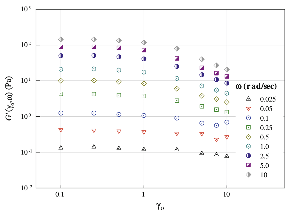
$\omega$ 에 대한 dynamic moduli를 plot하지 않고, $\gamma_0$ 에 대해 dynamic moduli를 plot한 결과를 보면, $\omega$ 가 커질수록 선형성의 편차가 커진다는 사실을 확인할 수 있다. 즉, $\gamma_{max}$ 는 $\omega$ 에 따라 달라진다.
그러므로 strain-controlled rheometer로 선형성 체크를 $\omega_{min} \le \omega \le \omega_{max}$ 에서 확인하기 위해 적어도 $\omega_{min}$ , $\omega_{max}$ 에서 2번의 amplitude sweep test를 통해 $\gamma_{max}$ 의 최소값을 골라야한다.

Complex Notation

모든 측정 가능한 양은 실수이다. 하지만 복소수를 사용하면 dynamic test의 결과를 알아보기 더 쉬워진다. complex strain을 $\gamma^*=\gamma_0 \exp(i\omega t)$ 라 하자. 그럼 $\gamma^*/dt=i\omega\gamma^*(t)$ 임을 알 수 있다. 이를 이용하여 BSP에 의해 complex stress를 구해보면 다음과 같다.

\begin{aligned} \sigma^*(t) &= i\omega\gamma_0 \int^t_{-\infin} G(t-\tau)e^{i\omega \tau}d\tau \\ Let\quad \xi &\equiv t-\tau\\ &= i\omega\gamma_0 \int^{\infin}_0 G(\xi)e^{i\omega(t-\xi)}d\tau \\ &= \gamma_0 e^{i\omega t}i\omega \int^{\infin}_0 G(\xi)e^{-i\omega\xi}d\tau \\ &= G^*(\omega)\gamma^*(t) \end{aligned}

그러면 $G^*(\omega)$ 는 다음과 같다.

\begin{aligned} G^*(\omega) &\equiv i\omega\int^{\infin}_0 G(t)e^{-i\omega t}dt\\ &= i\omega\int^{\infin}_0G(t)(\cos\omega t-i\sin\omega t)dt\\ &= i\omega\int^{\infin}_0G(t)\cos\omega t dt+\omega\int^{\infin}_0G(t)\sin\omega t dt\\ &=G^{\prime}(\omega) +iG^{\prime\prime}(\omega) \end{aligned}

Application of Laplace Transform

$G^*(\omega)$ 의 정의를 다시 보면 이는 라플라스 변환(laplace transform)의 형태와 동일하다는 것을 알 수 있다.

G^*(\omega)=\left[s\tilde G(s)\right]_{s=i\omega}

그리고 complex stress, $\sigma^*(t)$ 를 통해 다음과 같이 유도할 수 있다.

\begin{aligned} \sigma^*(t) &= \frac{G^*(\omega)}{i\omega}\left(i\omega\gamma^*(t)\right)\\ &= \frac{G^*(\omega)}{i\omega}\frac{d\gamma^*}{dt} \\ &= \eta^*(\omega)\frac{d\gamma^*}{dt} \end{aligned}

complex viscosity를 다음과 같이 정의할 수 있다.

\eta^*(\omega) \equiv \frac{G^*(\omega)}{i\omega}

전개하면 다음과 같은 dynamic moduli와 complex viscosity의 관계식을 얻을 수 있다.

\begin{aligned} \eta^*(\omega) &= \frac{G^{\prime}(\omega)+iG^{\prime\prime}(\omega)}{i\omega}\\ &= \eta^{\prime\prime}(\omega)-i\eta^{\prime}(\omega)\\\\ \eta^{\prime}(\omega) &\equiv \frac{G^{\prime\prime}(\omega)}{\omega}; \quad \eta^{\prime\prime}(\omega) \equiv \frac{G^{\prime}(\omega)}{\omega} \end{aligned}

또한 다음과 같은 결론을 얻을 수 있다.

\eta^*(\omega)=\tilde G(i\omega)

Application of Fourier Transform

$G(t)$ 에 퓨리에 변환(Fourier Transform)을 하면 다음과 같이 유도할 수 있다. 퓨리에 변환은 $\mathfrak{F}[G(t)]=\hat G(\omega)$ 으로 표시하자.

Fourier Transform of Real Function

\hat G(\omega) = \int^{\infin}_{-\infin}G(t)e^{-i\omega t}dt = \int^{\infin}_0 G(t)e^{-i\omega t}dt = \tilde G(i\omega) = \eta^*(\omega)

모든 실수 함수(real function)는 다음과 같이 표현할 수 있다.

f(t) = f_{even}(t) + f_{odd}(t);\quad \begin{cases} f_{even}(t) = \frac{f(t)+f(-t)}{2}\\ f_{odd}(t) = \frac{f(t)-f(-t)}{2} \end{cases}

even function의 퓨리에 변환은 다음과 같다.

\begin{aligned} \hat f_{even}(\omega) &= \int^{\infin}_{-\infin} f_{even}(t)\left[\cos\omega t - i \sin\omega t\right]dt \\ &= \int^{\infin}_{-\infin} f_{even}(t)\cos\omega t dt \\ &= 2\int^{\infin}_{0} f_{even}(t)\cos\omega t dt \end{aligned}

odd function의 퓨리에 변환은 다음과 같다.

\begin{aligned} \hat f_{odd}(\omega) &= \int^{\infin}_{-\infin} f_{even}(t)\left[\cos\omega t - i \sin\omega t\right]dt \\ &= -i\int^{\infin}_{-\infin} f_{odd}(t)\sin\omega t dt \\ &= -2i\int^{\infin}_{0} f_{odd}(t)\sin\omega t dt \end{aligned}

그러므로 모든 실수 함수에 대해서 퓨리에 변환은 다음과 같다.

\begin{aligned} \hat f(\omega) &= \hat f_{even}(\omega) + \hat f_{odd}(\omega)\\ &= 2\int^{\infin}_0 f_{even}(t)\cos\omega t dt - 2i \int^{\infin}_0 f_{odd}(t) \sin \omega t dt\\ \\ \hat f_{even}(\omega) &=2\int^{\infin}_0f_{even}(t)\cos\omega t dt;\quad \hat f_{odd}(\omega)=-2i \int^{\infin}_0 f_{odd}(t) \sin \omega t d \end{aligned}

Fourier Transform of $G(t)$

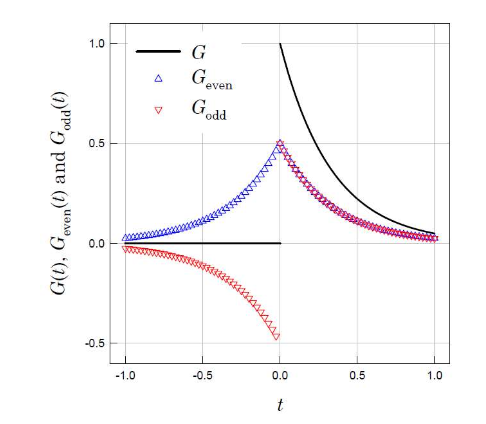
$G(t)$ 를 위와 같이 even function과 odd function으로 나누어 정의하자. 그럼 $t>0$ 에서 다음이 성립한다.

G_{even}(t) = G_{odd}(t) = \frac{1}{2}G(t)

그러므로 $G(t)$ 의 퓨리에 변환은 다음과 같다.

\begin{aligned} \hat G(\omega) &= \eta^*(\omega)\\ \hat G(\omega) &= 2\int^{\infin}_0 G_{even}(t)\cos\omega tdt-2i\int^{\infin}_0 G_{odd}(t)\sin\omega tdt\\ &= \eta^{\prime\prime}(\omega)-i\eta^{\prime}(\omega)\\ &= \frac{G^{\prime}(\omega)}{\omega}-i\frac{G^{\prime\prime}(\omega)}{\omega} \end{aligned}

퓨리에 변환의 정의에 의해 역 퓨리에 변환(inverse fourier transform)은 다음과 같다.

f(t) = \frac{1}{2\pi}\int^{\infin}_{-\infin}\hat f(\omega)e^{i\omega t}d\omega

그럼 다음과 같이 유도할 수 있다.

\begin{aligned} \frac{G^{\prime\prime}(\omega)}{\omega}&=\hat G_{even}(\omega)=2\int^{\infin}_0 G_{even}(t) \cos\omega t dt \\ G_{even}(t)&=\frac{1}{2\pi}\int^{\infin}_0 \frac{G^{\prime\prime}(\omega)}{\omega}e^{i\omega t} d\omega\\ &=\frac{1}{\pi}\int^{\infin}_0\frac{G^{\prime\prime}(\omega)}{\omega}\cos\omega t d\omega\\ G(t) &=\frac{2}{\pi}\int^{\infin}_0 \frac{G^{\prime\prime}(\omega)}{\omega}\cos\omega t d\omega \end{aligned}

마찬가지로 $\frac{G^{\prime}(\omega)}{\omega}$ 에 대해서도 구해보면,

G(t) = \frac{2}{\pi}\int^{\infin}_0 \frac{G^{\prime}(\omega)}{\omega}\sin\omega t d\omega

최종적으로 우리는 dynamic test로 구한 dynamic moduli, $G^{\prime}, G^{\prime\prime}$ 으로 static test로 구하는 relaxation modulus, $G(t)$ 를 구할 수 있다. 즉 static test에서 unit-step function의 완벽 재현에 어려움으로 짧은 시간 범위에서 정확한 $G(t)$ 를 구할 수 없었지만, dynamic test의 결과와 퓨리에 변환을 적절히 사용하여 정확한 $G(t)$ 를 구할 수 있다!

Terminal Behavior

dynamic test에서 주파수가 매우 낮다면, 우리는 다음과 같은 근사를 할 수 있다.

\sin \omega t \approx \omega t;\quad \cos \omega t \approx 1

그럼 dynamic moduli는 다음과 같이 근사된다.

G^{\prime}(\omega) \approx \omega^2 \int^{\infin}_0 tG(t) dt;\quad G^{\prime\prime}(\omega) \approx \omega \int^{\infin}_0 G(t)dt

낮은 주파수 영역에서 zero-shear viscoisty, mean relaxation time, steady state compiance를 다음과 같이 새로 정의하자.

\begin{aligned} \eta_0 &\equiv \int^{\infin}_0 G(t)dt\\ \bar \lambda &\equiv \frac{1}{\eta_0}\int^{\infin}_0 tG(t) dt\\ J^0_e &\equiv \frac{\bar \lambda}{\eta_0} \end{aligned}

이제 $J^0_e$ 와 $\eta_0$ 를 구해보자.

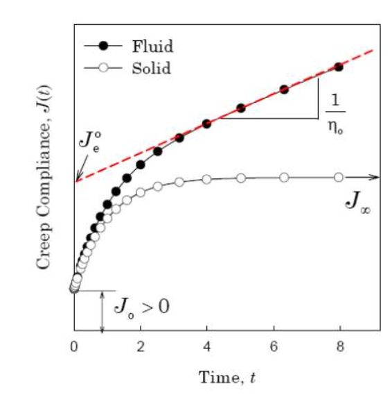
creep test의 실험 결과에서 빨간색 직선을 일차함수로 근사해보자.

J(t) \approx at + b

빨간색 직선의 기울기가 왜 $1/\eta_0$ 이고 $y$ 절편이 $J^0_e$ 인지 다음의 유도를 통해 알 수 있다.

\begin{aligned} \tilde J(s) &\approx \mathfrak{L}[at+b] = \frac{a}{s^2}+\frac{b}{s}=\frac{bs+a}{s^2}\\ s\tilde G(s) &= \frac{1}{s \tilde J(s)} = \frac{s}{bs+a}\\ \\ G^*(\omega) &= \left[s\tilde G(s)\right]_{s=i\omega}\\ G^*(\omega) &= G^{\prime}(\omega) + iG^{\prime\prime}(\omega) \approx \frac{i\omega}{ib\omega+a} \\&= \frac{b\omega^2}{a^2 + b^2\omega^2} + i \frac{a\omega}{a^2 + b^2\omega} \\ \\ At\; \omega &\ll 1\\ G^{\prime}(\omega) &\approx \frac{b}{a^2}\omega^2 = J^0_e\eta^2_0\omega^2;\quad G^{\prime\prime}(\omega) \approx \frac{1}{a}\omega = \eta_0\omega \end{aligned}

그러므로

a=\frac{1}{\eta_0};\quad\quad b=J^0_e

임을 알 수 있다.

Waiting time for Dynamic Test

실제로 strain-controlled rheometer에서 실험해보면, 일정 시간 후에 stress의 진폭이 시간에 거의 독립적임을 알 수 있다. 이를 stationary response라고 한다.

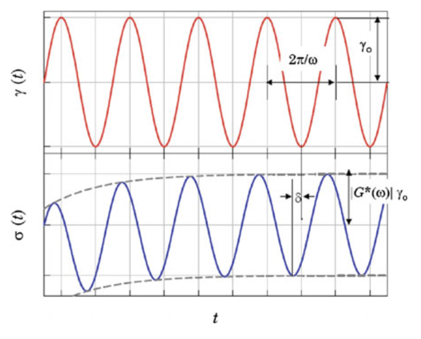
즉, rheometer는 stationary response, $\sigma(t)$ 를 stress의 진폭, $\sigma_0$ 과 phase difference, $\delta(\omega)$ 를 통해 다음과 같이 나타낸다.

\begin{aligned} \sigma_0 &= |G^*(\omega)|\gamma_0 \\ \sigma(t) &= \sigma_0 \left[\sin \omega t + \delta(\omega)\right] \end{aligned}

위의 $\sigma(t)$ 는 BSP로 구한

\sigma(t) = G^{\prime}(\omega) \gamma(t) + \frac{G^{\prime\prime}\omega}{\omega}\dot \gamma(t)

와 같아야 한다. dyanamic test에서 stationary response로 나타나는 $\sigma(t)$ 를 삼각함수 덧셈공식으로 전개하여 BSP로 유도한 $\sigma(t)$ 와 비교해보면 다음과 같은 결론을 얻을 수 있다.

G^{\prime}(\omega) = |G^*(\omega)|\cos\delta(\omega);\quad\quad G^{\prime\prime}(\omega)=|G^*(\omega)|\sin\delta(\omega)

jmt

고분자/컴공

이전 포스트

[Linear Viscoelasticity] 03. Static Test

다음 포스트

[Linear Viscoelasticity] 04. Dynamic Test

선형점탄성(Linear Viscoelasticity)

Dynamic Test

Dynamic Moduli

Linearity Check