축구선수 이적시장 분석 - 기초 통계값

1. 기초 통계값

1.1 평균, 중앙값, 최빈값 비교

정규분포 그래프를 사용해 데이터의 구성과 대표값을 파악합니다.

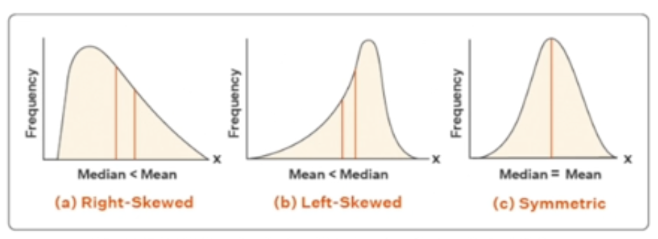
1.1.1 Left Skew

평균(mean) < 중앙값(median) < 최빈값(mode)

[ 1, 3, 5, 7 ,10, 10, 10 ] 
평균 : 6.5
중앙값 : 7
최빈값 : 10

데이터 구성을 확인했을 때, 값이 큰 데이터가 많이 분포하고 있습니다.

1.1.2 Normal Distribution

평균(mean) = 중앙값(median) = 최빈값(mode)

예시: [ 4, 6, 7, 7 ,7 ,8 ,10 ] 

평균 : 7
중앙값 : 7
최빈값 : 7

데이터가 골고루 분포하고 있습니다.

1.1.3 Right skew

평균(mean) > 중앙값(median) > 최빈값(mode)

예시: [ 1, 1, 1, 2, 2, 5, 6 ] 
평균 : 2.5
중앙값 : 2
최빈값 : 1

작은 값을 갖는 데이터가 많고 값이 큰 데이터는 적습니다.

중앙값을 기준으로 반은 더 같거나 작고, 반은 더 같거나 큰 값을 갖습니다.

pd.options.display.float_format = '{:.3f}'.format

players_valuations['market_value_in_eur'].describe()

mean_ = players_valuations['market_value_in_eur'].mean()
over_mean = len(players_valuations[players_valuations['market_value_in_eur'] > mean_])
total = len(players_valuations)
print(f'percentile of player over mean value: {over_mean/total * 100: .2f}%')

players_with_val = pd.merge(players, players_valuations, on='player_id')
players_with_val[players_with_val['last_name'] == 'Son'].tail()

players_with_val['date']

# 결과값:
# 0         2004-10-04
# 1         2005-10-17
# 2         2006-06-14
# 3         2007-04-24
# 4         2007-09-01

# lambda x: int(x[:4])는 년도만 슬라이싱하기
players_with_val['year'] = players_with_val['date'].apply(lambda x: int(x[:4]))

players_with_val.drop_duplicates(['player_id', 'dateyear'], keep='last', inplace=True)
players_with_val[players_with_val['last_name'] == 'Son']

players_with_val_2022['market_value_in_eur'] = players_with_val_2022['market_value_in_eur'].rank(method='min', ascending=False)