오랜만에 쓰는... 공부글...

패키지부터 설치해준다.

Packages

import numpy as np

간단한 원리를 알아보는거라 넘파이만 사용한다.

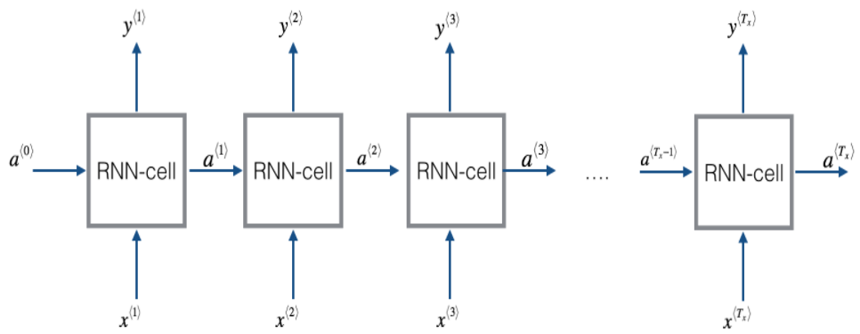
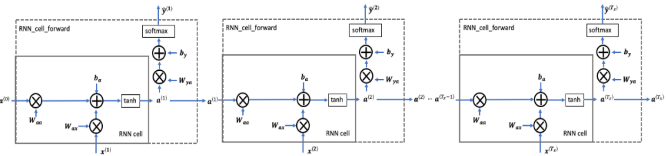
input Tx와 output Ty의 길이가 같다면, 기본적인 RNN모델은 아래와 같이 생겼다.

RNN의 single sell구조를 확인해보자.

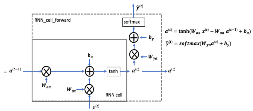
가장 기본적인 RNN cell이다. x< t>(현재 input)와 a< t-1>(과거 정보를 갖고있는 hidden state)을 input으로 가지고 a< t>(다음 RNN cell에게 전달)를 출력한다.

위 RNN cell forward 코드를 작성해보자.

RNN cell forward

def rnn_cell_forward(xt, a_prev, parameters):
    Wax = parameters["Wax"]
    Waa = parameters["Waa"]
    Wya = parameters["Wya"]
    ba = parameters["ba"]
    by = parameters["by"]
    
    # compute next activation state using the formula given above
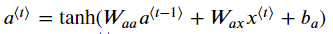
    a_next = np.tanh(np.dot(Waa,a_prev) + np.dot(Wax,xt) + ba)
    # compute output of the current cell using the formula given above
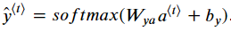
    yt_pred = softmax(np.dot(Wya,a_next) + by)
    
    # store values you need for backward propagation in cache
    cache = (a_next, a_prev, xt, parameters)
    
    return a_next, yt_pred, cache

위 코드에서 a_next = np.tanh(np.dot(Waa,a_prev) + np.dot(Wax,xt) + ba)는 아래 식을 이용해 hidden state를 tanh activation함수로 계산해준 값이다.

두번째로 예측값을 위해 아래 식을 사용해서 yt_pred = softmax(np.dot(Wya,a_next) + by)을 작성해주었다.

이후에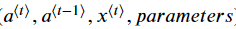
값들을 cache에 저장하고 a_next, yt_pred, cache를 반환한다.

이번에는 하나의 셀을 가지고 하지않고, 연속된 셀들을 묶어 rnn forward 함수를 구현해보자.

위에서 cell을 여러개 이어놓은 모습일 것이다.

RNN forward

def rnn_forward(x, a0, parameters):
    # Initialize "caches" which will contain the list of all caches
    caches = []
    
    # Retrieve dimensions from shapes of x and parameters["Wya"]
    n_x, m, T_x = x.shape
    n_y, n_a = parameters["Wya"].shape
    
    # initialize "a" and "y_pred" with zeros 
    a = np.zeros((n_a, m, T_x))
    y_pred = np.zeros((n_y, m, T_x))
    
    # Initialize a_next 
    a_next = a0
    
    # loop over all time-steps
    for t in range(T_x):
        # Update next hidden state, compute the prediction, get the cache 
        a_next, yt_pred, cache = rnn_cell_forward(x[:,:,t], a_next, parameters)
        
        # Save the value of the new "next" hidden state in a
        a[:,:,t] = a_next
        
        # Save the value of the prediction in y 
        y_pred[:,:,t] = yt_pred
        
        # Append "cache" to "caches" 
        caches.append(cache)
        
    # store values needed for backward propagation in cache
    caches = (caches, x)
    
    return a, y_pred, caches

shape of a:

shape of y_pred:

a = np.zeros((n_a, m, T_x))와
y_pred = np.zeros((n_y, m, T_x))로 a와 yhat array를 만들어준다. a는 RNN으로 계산된 hidden state를 저장하고, yhat은 예측값을 저장한다.

a_next를 initial hidden state 인 a0과 같게 해주어 초기화를 해 준 후,
모든 타임 스탭 t에 대해 아래 반복문을 돌린다.

• 위에 구했던 rnn_cell_forward함수의 리턴값에 대해 hidden state과 예측값, cache를 저장해준다.
• 2D hidden state를 3D tensor인 a의 t번째 자리에 저장한다. 여기서 a는 크기를 가지고 있다.
• 예측값yt_pred을 3D tensor인 y_pred에 저장한다.
  여기서 yt_pred는
  y_pred는
  크기를 갖는다.
• cache값을 caches에 저장한다.

루프문을 반복한 후 3D tensor a와 yhat, caches를 반환한다.

RNN의 forward propagation을 완성했다.
다음으로는 LSTM network cell에 대해 알아보자.

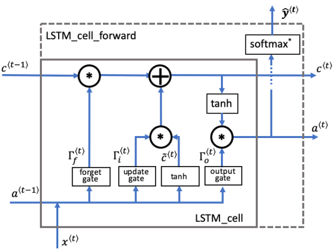
위와 같은 방법으로 하나의 셀에 대한 함수를 만들어보자.

LSTM cell forward

def lstm_cell_forward(xt, a_prev, c_prev, parameters):
    # Retrieve parameters from "parameters"
    Wf = parameters["Wf"] # forget gate weight
    bf = parameters["bf"]
    Wi = parameters["Wi"] # update gate weight (notice the variable name)
    bi = parameters["bi"] # (notice the variable name)
    Wc = parameters["Wc"] # candidate value weight
    bc = parameters["bc"]
    Wo = parameters["Wo"] # output gate weight
    bo = parameters["bo"]
    Wy = parameters["Wy"] # prediction weight
    by = parameters["by"]
    
    # Retrieve dimensions from shapes of xt and Wy
    n_x, m = xt.shape
    n_y, n_a = Wy.shape

    # Concatenate a_prev and xt 
    concat = np.concatenate((a_prev, xt))

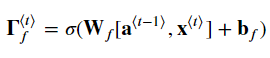
    # Compute values for ft, it, cct, c_next, ot, a_next using the formulas given figure (4) 
    ft = sigmoid(np.dot(Wf,concat) + bf)
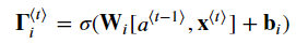
    it = sigmoid(np.dot(Wi,concat) + bi)
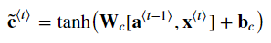
    cct = np.tanh(np.dot(Wc,concat) + bc)
    c_next = ft * c_prev + it * cct
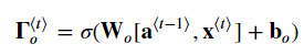
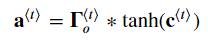
    ot = sigmoid(np.dot(Wo,concat) + bo)
    a_next = ot * np.tanh(c_next)
    
    # Compute prediction of the LSTM cell 
    yt_pred = softmax(np.dot(Wy, a_next) + by)


    # store values needed for backward propagation in cache
    cache = (a_next, c_next, a_prev, c_prev, ft, it, cct, ot, xt, parameters)

    return a_next, c_next, yt_pred, cache

a_prev, xt를 Concat하는 방법은 np.concatenate로 간단하게 구현할 수 있다.

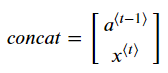
위와 같은 sigle matrix가 생성된다.

아래 식 여섯개를 구현한다.






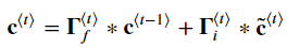
이제 게이트와 히든스테이트, 셀 게이트를 계산했다.
마지막으로 예측값softmax(np.dot(Wy, a_next) + by)을 계산해주면 된다.

셀을 구했다면 연속된 루프를 사용하여 전체 process를 구현해보자.

LSTM forward pass

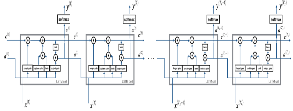
연속된 시간에 따른 LSTM모습이다.
위에서 만든 lstm_cell_forward를 이용해 구현해보자.

def lstm_forward(x, a0, parameters):
    # Initialize "caches", which will track the list of all the caches
    caches = []
    
    Wy = parameters['Wy'] # saving parameters['Wy'] in a local variable in case students use Wy instead of parameters['Wy']
    # Retrieve dimensions from shapes of x and parameters['Wy'] 
    n_x, m, T_x = x.shape
    n_y, n_a = Wy.shape
    
    # initialize "a", "c" and "y" with zeros 
    a = np.zeros((n_a, m, T_x))
    c = a.copy()
    y = np.zeros((n_y, m, T_x))
    
    # Initialize a_next and c_next
    a_next = a0
    c_next = np.zeros(a_next.shape)
    
    # loop over all time-steps
    for t in range(T_x):
        # Get the 2D slice 'xt' from the 3D input 'x' at time step 't'
        xt = x[:,:,t]
        # Update next hidden state, next memory state, compute the prediction, get the cache 
        a_next, c_next, yt, cache = lstm_cell_forward(xt, a_next, c_next, parameters)
        
        # Save the value of the new "next" hidden state in a 
        a[:,:,t] = a_next
        
        # Save the value of the next cell state 
        c[:,:,t]  = c_next
        
        # Save the value of the prediction in y 
        y[:,:,t] = yt
        
        # Append the cache into caches
        caches.append(cache)

    # store values needed for backward propagation in cache
    caches = (caches, x)

    return a, y, c, caches

x와 parameter로부터 nx, na, ny, m, Tx의 차원을 얻는다.
n_x, m, T_x = x.shape
n_y, n_a = Wy.shape
a, c, y를 초기화해준다.
a< t>, c< t>초기화.
모든 time step에 대해 lstm_cell_forward 입혀주고 hidden state, cell state, prediction을 3D 안에 넣어준다.
caches에 cache넣는다.

여기서 RNN과 LSTM의 forward pass설명을 마친다.