
이번에는 이진 분류를 해 볼 것이다.
이진 분류란, 어떤 데이터에 관해서 0이나 1로 분류되는 것을 말한다.
tensor에서 제공하는 IMDB 리뷰 데이터를 가지고 분류해보자.
Packages
from tensorflow.keras.datasets import imdb
%matplotlib inline
import matplotlib.pyplot as plt
import numpy as np
데이터를 각각 X_train, y_train, X_test, y_test에 저장하자.
(X_train, y_train), (X_test, y_test) = imdb.load_data()궁금했던 것들을 확인해보자.
print(len(X_train))    #트레인 세트의 크기     #25000
print(len(X_test))     #테스트 세트의 크기     #25000
print(max(y_train)+1)  #트레인 세트 라벨 크기  #2
print(y_train[0])      #첫번째 트레인 세트 라벨 이름 #1
print(y_train[1])      #두번째 트레인 세트 라벨 이름 #0
print(X_train[0])      #첫번째 데이터 내용
마지막 첫번째 데이터 내용은
[1, 14, 22, 16, 43, 530, 973, 1622, 1385, 65, 458, 4468, 66, 3941, 4, 173, 36, 256, 5, 25, 100, 43,
이런 식으로 숫자로 나온다. 이미 전처리가 되어있는 모습이다.
이번엔 각 리뷰 안에 최대 길이 리뷰와 전체 리뷰의 평균 길이를 확인해보자.
len_result = [len(s) for s in X_train]
print(np.max(len_result))
print(np.mean(len_result))
최대 길이는 2494, 평균 길이는 236.7정도가 나온다.
500정도로 잘라주면 괜찮을 듯 하다.
모델을 만들어보자!
Build model
Packages
from tensorflow.keras.datasets import imdb
from tensorflow.keras.preprocessing.sequence import pad_sequences
from tensorflow.keras.models import Sequential
from tensorflow.keras.layers import Dense, LSTM, Embedding
from tensorflow.keras.callbacks import EarlyStopping, ModelCheckpoint
from tensorflow.keras.models import load_model
데이터를 다시 불러와준다.
그리고 전체 데이터에 대해서 작업하는데 시간이 많이 소요되므로 사용 빈도수가 높은 5000개의 단어만 가져온다.
(X_train, y_train), (X_test, y_test) = imdb.load_data(num_words=5000)아까 위에서 최대 길이와 평균길이를 보고 500정도로 잘라줘야겠다고 얘기했었다. 패딩해주자.
max_len = 500
X_train = pad_sequences(X_train, maxlen=max_len)
X_test = pad_sequences(X_test, maxlen=max_len)
모델을 만들어보자.
이진 분류이기 때문에 활성함수는 sigmoid함수를 사용한다.
model = Sequential()
model.add(Embedding(5000, 120))
model.add(LSTM(120))
model.add(Dense(1, activation='sigmoid'))
학습시켜주자
model.compile(loss='binary_crossentropy', optimizer='adam', metrics=['acc'])
history=model.fit(X_train, y_train, validation_data=(X_test,y_test), epochs=20, batch_size=64)
Analysis
scores = model.evaluate(X_test, y_test)
print('acc: %.4ff%%'% (scores[1]*100))
약 83%의 정확도가 나온다.
이제 그래프로 나타내보자.
위에서 정의했던 history를 보면 많은 key들이 있는데 어떤 것들이 있는지 확인해보자.
history_dict = history.history
history_dict.keys()
dict_keys(['loss', 'acc', 'val_loss', 'val_acc'])
이런 것들을 뽑아올 수 있다.
loss와 val_loss를 가지고 그래프를 그려보자.
import matplotlib.pyplot as plt

loss=history_dict['loss']
val_loss=history_dict['val_loss']

epochs=range(1, len(acc)+1)

plt.plot(epochs, loss, 'bo', label='Training loss')
plt.plot(epochs, val_loss, 'b', label='Validation loss')
plt.title('Training and validation loss')
plt.xlabel('Epochs')
plt.ylabel('Loss')
plt.legend()
plt.show()
acc와 val_acc에 대해서도 그래프를 그려보자.
첫번째 줄에 초기화를 해 준 부분을 제외하면 아래는 비슷하다.
plt.clf()

plt.plot(epochs, acc, 'bo', label='Training acc')
plt.plot(epochs, val_acc, 'b', label= 'valadation acc')
plt.title('Training and validation accuracy')
plt.xlabel('Epochs')
plt.ylabel('Accuracy')
plt.legend()

plt.show()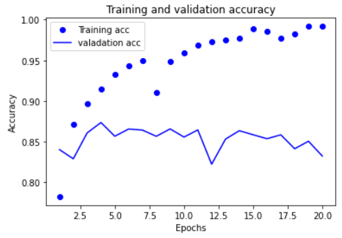
훈련 데이터에 대해서는 epochs가 증가하면서 정확도가 증가한다. 하지만 val데이터에 대해서는 그렇게 이상적인 결과는 아닌 것 같다. 5번째 epochs부터 오히려 정확도가 떨어진다.
그래서 epochs를 4로 낮춰봤다.
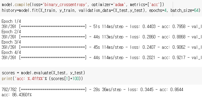
그랬더니 86%의 정확도를 얻었다.