이전 글에서 의도분류에 대해서 설명하고, 영어 버전으로 실습을 해 보았다. 이번에는 한국어로 실습을 해보도록 하자.
그리고, 이전에는 멀티 커널 CNN으로 모델을 구축했었는데, 이번에는 LSTM으로 모델을 구축해볼 것이다.

패키지를 불러와주자.

Packages

이번에는 한국어에 대해 전처리를 진행하기 때문에 후에 Okt를 사용하기 위해서 konlpy를 불러와준다.

!pip install konlpy

이후에 matplotlib에서 그리는 그래프에서 한글이 깨지는 것을 방지하기 위해 아래 코드를 실행해주자.

import matplotlib.pyplot as plt
import matplotlib as mpl
import matplotlib.font_manager as fm

%config InlineBackend.figure_format = 'retina'

!apt -qq -y install fonts-nanum > /dev/null

fontpath = '/usr/share/fonts/truetype/nanum/NanumBarungothic.ttf'
font = fm.FontProperties(fname=fontpath, size=9)
mpl.font_manager._rebuild()
mpl.pyplot.rc('font', family='NanumBarunGothic')

위 코드를 실행했다면 런타임을 다시 시작해서 코드를 재실행해주자.
마지막으로 패키지를 불러와준다.

import urllib.request
import pandas as pd
import numpy as np
import matplotlib.pyplot as plt
from konlpy.tag import Okt
from tensorflow.keras.preprocessing.text import Tokenizer
from tensorflow.keras.preprocessing.sequence import pad_sequences
from sklearn import preprocessing

데이터를 가져오자.

Import Data

urllib.request.urlretrieve("https://raw.githubusercontent.com/hukim1112/comment_classifier/master/train_intent.csv", filename="train_intent.csv")

전처리 과정을 해주자.

Data Preprocessing

파일 안에 내용을 확인해보기 위해서, 파일을 읽고 앞에 20개 내용을 출력해보자.

df = pd.read_csv('train_intent.csv')
df.sample(20)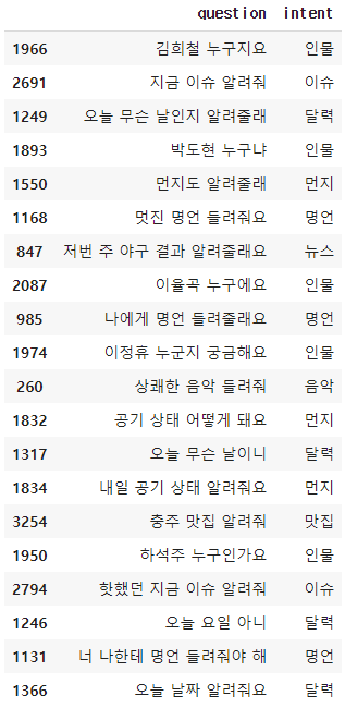

key()값을 확인해보면 question 과 intent값이 있다.
plot으로 각 카테고리에서 개수를 확인해보자.

df['intent'].value_counts().plot(kind = 'bar')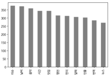

아래 명령을 돌리면 정확한 개수를 확인할 수 있다.

df.groupby('intent').size().reset_index(name='count')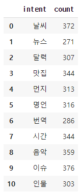

비어있는 값이 있는지 확인해주자.

df.isnull().values.any()

없으니까 이대로 진행하자.
Okt를 불러와주고 단어를 쪼개주자.

okt = Okt()

X_train = []
for sentence in df.question:
  temp_X = []
  temp_X = okt.morphs(sentence)
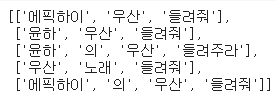
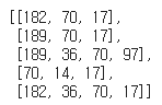
  X_train.append(temp_X)

X_train의 앞에 다섯개 값을 확인해보면 아래와 같은 결과를 얻는다.

토큰화를 해 보자.

Tokenization

tokenizer = Tokenizer()

tokenizer.fit_on_texts(X_train)

X_train = tokenizer.texts_to_sequences(X_train)

X_train[:5] 이 명령으로 앞에 다섯개 샘플 내용을 확인할 수 있다.

문장들이 숫자로 변환되었다.
tokenizer.word_index이걸로 전체 단어 인덱스 표를 확인할 수 있다. 너무 기니 생략하겠다.

Padding

패딩을 위해 전체 길이와, 최대 길이, 평균 길이를 구해보자.

vocab_size = len(tokenizer.word_index)+1
vocab_size

전체 길이는 1402개가 나온다.

max(len(l) for l in X_train)

최대 길이는 10,

sum(map(len, X_train))/len(X_train)

평균 길이는 4.11이 나온다.
표로 확인해보자.

plt.hist([len(s) for s in X_train], bins=17, color='grey')
plt.xlabel('length')
plt.ylabel('sample num')
plt.show()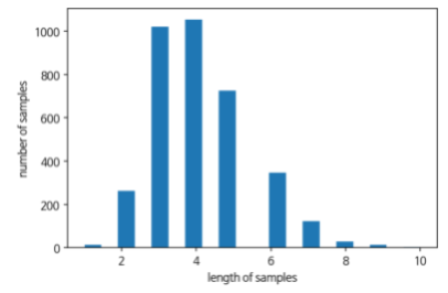

max_len은 아마 10으로 해도 괜찮을 것 같다.
10을 기준으로 패딩해주자.

max_len = 10
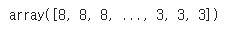
X_train = pad_sequences(X_train, maxlen = max_len, padding='post')
X_train[:5]

마지막 줄을 출력하면

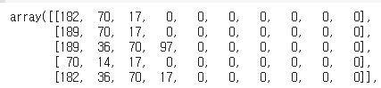
이런 결과를 얻을 수 있다. 빈칸에 0이 채워진 모습이다.

이제 라벨에도 인코딩을 해주자.

idx_encode = preprocessing.LabelEncoder()
idx_encode.fit(df['intent'])

y_train = idx_encode.transform(df['intent'])

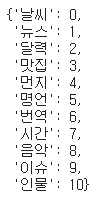
label_idx = dict(zip(list(idx_encode.classes_), idx_encode.transform(list(idx_encode.classes_))))

label_idx를 출력해보면 각 카테고리가 숫자로 레이블되었다.

이제 위 내용을 실제 데이터에도 도입시켜야 한다.
실제 데이터 상에서도 레이블을 숫자로 바꿔주자.

idx_label = {}
for key, value in label_idx.items():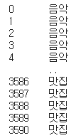
  idx_label[value] = key

y_train을 출력해보면

글자 대신 숫자가 표시된다.
(참고로 이전에는 ,

이런식으로 표시됐었다.)

모델링 해보자.

Build Model

Packages

from tensorflow.keras.layers import Embedding, Dense, LSTM
from tensorflow.keras.models import Sequential
from tensorflow.keras.models import load_model

LSTM모델을 만들어주자.

model = Sequential()
model.add(Embedding(vocab_size, 64))
model.add(LSTM(256))
model.add(Dense(len(label_idx), activation='softmax'))

model.compile(optimizer='rmsprop', loss='sparse_categorical_crossentropy', metrics=['acc'])
history=model.fit(X_train, y_train, epochs=15, batch_size=64)

약 99% 100%정도의 정확도가 나온다.
그래프로 확인해보자.

epochs = range(1, len(history.history['acc']) + 1)
plt.plot(epochs, history.history['acc'])

plt.title('model accuracy')
plt.ylabel('accuracy')
plt.xlabel('epochs')
plt.legend(['train'], loc='lower right')
plt.show()

epochs = range(1, len(history.history['loss']) + 1)
plt.plot(epochs, history.history['loss'])

plt.title('model loss')
plt.ylabel('loss')
plt.xlabel('epochs')
plt.legend(['train'], loc='upper right')
plt.show()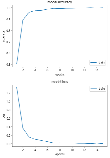

나중에 이 데이터를 잘 믹스해서 train데이터와 val데이터로 나눠서 실험해보고 싶다.

Evaluate

이제 원하는 문장을 넣었을 때 의도분류를 제대로 하는지 확인해보자.
해당하는 함수를 만들어준다.

def question_processing(sentences):
  inputs = []
  for sentence in sentences : 
    sentence = okt.morphs(sentence)
    encoded = tokenizer.texts_to_sequences([sentence])
    inputs.append(encoded[0])
  padded_inputs = pad_sequences(inputs, maxlen=max_len, padding='post')
  return padded_inputs

input_sentence = question_processing(['포스트잇이 중국어로 뭐야'])

prediction = np.argmax(model2.predict(input_sentence), axis = 1)

을 입력하면 해당하는 인덱스 넘버가 뜬다.
숫자가 아닌 글자를 원하기 때문에 아래 코드를 다시 실행해주자.

for p in prediction:
  print(idx_label[p])

언어가 뜬다.

Add New Data

이번에는 새로운 문장을 라벨링하여 원래 데이터에 추가해주자.

nouns = ['키보드', '아이패드', '맥북']
def question_generator(nouns):
  question = []
  for noun in nouns :
    s1 = noun+'가 아랍어로 뭐야?'
    s2 = noun+'가 일본어로 뭐야?'
    s3 = noun+'가 이탈리아어로 뭐야?'
    question = question+[s1,s2,s3]
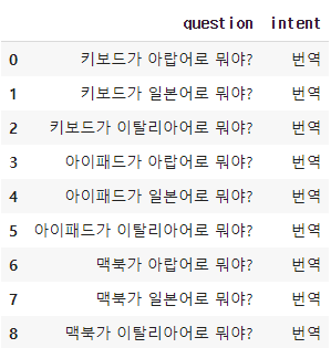
  return question

question = question_generator(nouns)

그리고 question을 출력해서 확인해보자.

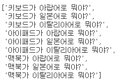
위 아홉 문장을 추가해 줄 것이다.
번역이라는 intent안에 위 문장들을 추가해주자.

new_data = {'question':question, 'intent':['번역']*len(question)}
add_df = pd.DataFrame(new_data, columns=('question','intent'))

add_df를 출력하여 확인해준다.

new_df의 길이를 확인해보면 이전에 가지고 있던 3591개의 데이터에서 9개가 추가된 3600개가 된 것을 확인할 수 있다.

다시 위에 okt에 넣는 과정부터 토큰화, 패딩 등 전처리 작업을 거친 후 다시 학습시킨다.

input_sentence = question_processing(['아이패드가 일본어로 뭐임'])

prediction = np.argmax(model.predict(input_sentence), axis = 1)
prediction

방금 우리가 학습시켰던 문장을 넣으면

for p in prediction:
  print(idx_label[p])

인텐트 값으로 넣었던 값이 출력된다.
여기서 설명을 마무리한다.