이번 글에서는 넘파이를 사용하지 않고 프레임워크를 통해 더 간단하게 모델을 구축할 수 있는 방법을 소개하겠다.

먼저 패키지를 다운받아주자.

import h5py
import numpy as np
import tensorflow as tf
import matplotlib.pyplot as plt
from tensorflow.python.framework.ops import EagerTensor
from tensorflow.python.ops.resource_variable_ops import ResourceVariable
import time

텐서플로우 2.3 버전을 사용할 것이기 때문에, 아래 코드를 통해 버전을 확인해주자.

tf.__version__

이하 버전이라면 다운받아 사용하면 된다.
다운받아 실행 할 때에는 실행을 한 후, 런타임 다시 실행 버튼으로 꼭 다시 실행시켜주자.

Basic Optimization with GradientTape

Tensorflow는 기본적으로 GradientTape에 그래프 값을 저장하면서 미분값을 계산할 수 있는 능력을 가지고 있다. 이것을 구현해보자.

여기서 Hand sign data set을 사용할 것이고, 이미지는 64x64x3의 크기를 가지고 있다. 이 데이터셋을 가져와주자.

train_dataset = h5py.File('datasets/train_signs.h5', "r")
test_dataset = h5py.File('datasets/test_signs.h5', "r")

각각의 변수에 저장해준다.

x_train = tf.data.Dataset.from_tensor_slices(train_dataset['train_set_x'])
y_train = tf.data.Dataset.from_tensor_slices(train_dataset['train_set_y'])

x_test = tf.data.Dataset.from_tensor_slices(test_dataset['test_set_x'])
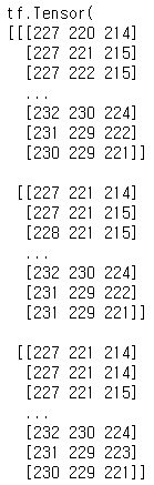
y_test = tf.data.Dataset.from_tensor_slices(test_dataset['test_set_y'])

여기서 x_train의 내용을 확인하려고 그대로 출력하게되면

내용에 접근이 불가능하다. 대신 iter와 next를 이용해서 파이썬 iterator를 만들어주면 가능하다.

print(next(iter(x_train)))

위 코드를 실행시키면 내용을 확인할 수 있다.

y_train 안에 있는 레이블을 확인해보자.

unique_labels = set()
for element in y_train:
    unique_labels.add(element.numpy())
print(unique_labels)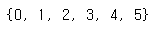

0부터 5까지의 태그가 있다.
이미지를 확인해보자.

images_iter = iter(x_train)
labels_iter = iter(y_train)
plt.figure(figsize=(10, 10))
for i in range(25):
    ax = plt.subplot(5, 5, i + 1)
    plt.imshow(next(images_iter).numpy().astype("uint8"))
    plt.title(next(labels_iter).numpy().astype("uint8"))
    plt.axis("off")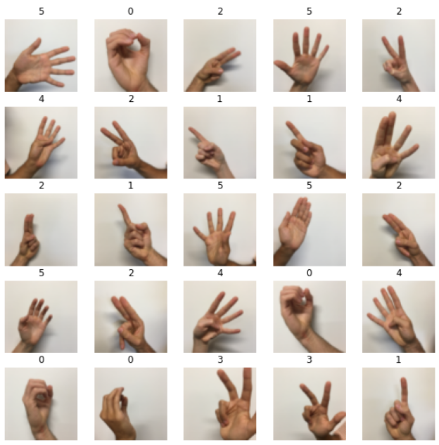

모든 이미지를 tf.cast함수를 사용하여 float32형태로 바꿔준 후 reshape해 주는 함수를 만들어주자.

def normalize(image):
    image = tf.cast(image, tf.float32) / 255.0
    image = tf.reshape(image, [-1,])
    return image

Tensorflow에서는 map함수를 이용하여 각 원소에 주어진 함수(여기서는 normalize를 적용하여 새로운 데이터셋을 생성할 수 있다.
각각 new_train과 new_test안에 저장해준다.

new_train = x_train.map(normalize)
new_test = x_test.map(normalize)

개별 요소의 유형을 확인할 수 있는 element_spec함수를 이용하여 shape를 확인해보자.

new_train.element_spec

다시 new_train을 출력해보면,

print(next(iter(new_train)))

모양이 달라져있다.

Linear Function

이번에는 아래 식을 계산하는 연습을 해 보자.

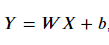
이번 예제에서는 X를 shape of (3,1)로, W를 (4,3), b를 (4,1)로 만들어보자.
아래처럼 함수를 만들면 된다.

def linear_function():
    np.random.seed(1)
    
    X = tf.constant(np.random.randn(3,1), name = "X")
    W = tf.constant(np.random.randn(4,3), name = "W")
    b = tf.constant(np.random.randn(4,1), name = "b")
    Y = tf.add(tf.matmul(W, X),b)
    
    return Y

tf.Variable은 상태를 수정할 수 있지만,
tf.constant를 사용하게 되면 이제 수정할 수 없게 된다.

X, W, b를 만들어 준 후, 식에 맞춰 Y값을 적어주었다.

Computing Sigmoid

이번엔 sigmoid함수를 구현해보자.

def sigmoid(z):
    z = tf.cast(z, tf.float32)
    a = tf.keras.activations.sigmoid(z)
    return a

One-hot Encoding

원 핫 인코딩에 대해서는 이전 글에서도 많이 설명을 했었다.

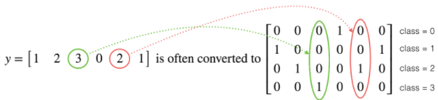
해당하는 숫자에 1을 표시하고 나머지 칸에 다 0으로 채워주는 방식이다.
텐서플로우에서는 tf.one_hot이라는 함수를 제공한다. 사이트에서 확인할 수 있다.
이를 사용해서 함수를 빌드해보자.

def one_hot_matrix(label, depth=6):
    one_hot = tf.reshape(tf.one_hot(label, depth, axis=0),(depth,))
    return one_hot

y_test와 y_train을 이 함수에 통과시킨 결과물을 new_y_test와 new_y_train에 넣어주자.

Initialize parameters

파라미터들을 초기화시켜줄 차례이다.
각자의 크기에 맞춰 tf.Variable을 사용하여 초기화 시켜준다.
파라미터들은 값이 계속 변하기 때문에 tf.Variable을 사용해 주어야 한다.

def initialize_parameters():
    initializer = tf.keras.initializers.GlorotNormal(seed=1)   
    
    W1 = tf.Variable(initializer(shape=[25,12288]))
    b1 = tf.Variable(initializer(shape=[25,1]))
    W2 = tf.Variable(initializer(shape=[12,25]))
    b2 = tf.Variable(initializer(shape=[12,1]))
    W3 = tf.Variable(initializer(shape=[6,12]))
    b3 = tf.Variable(initializer(shape=[6,1]))
    
    parameters = {"W1": W1,
                  "b1": b1,
                  "W2": W2,
                  "b2": b2,
                  "W3": W3,
                  "b3": b3}
    
    return parameters

이 함수를 parametes에 넣어주자.

parameters = initialize_parameters()

Build NN

앞서 말했듯이 tensorflow의 가장 큰 장점은 forward_propagation만 만들어놓으면 뒤에 부분은 알아서 해준다는 것이다.

Forward Propagation

LINEAR -> RELU -> LINEAR -> RELU -> LINEAR 의 모델을 만들어주자.

def forward_propagation(X, parameters):
    W1 = parameters['W1']
    b1 = parameters['b1']
    W2 = parameters['W2']
    b2 = parameters['b2']
    W3 = parameters['W3']
    b3 = parameters['b3']
    
    Z1 = tf.add(tf.matmul(W1, X),b1)
    A1 = tf.keras.activations.relu(Z1)
    Z2 = tf.add(tf.matmul(W2, A1),b2)
    A2 = tf.keras.activations.relu(Z2)
    Z3 = tf.add(tf.matmul(W3, A2),b3)
    
    return Z3

Compute Cost

def compute_cost(logits, labels):
    cost = tf.reduce_mean(tf.keras.losses.categorical_crossentropy(tf.transpose(labels), tf.transpose(logits), from_logits = True))
    
    return cost

위 함수에서 categorical crossentropy loss를 계산해주는 tf.keras.losses.categorical_crossentropy가 사용되었다.
안에 인자 중에서 from_logits는 모델의 출력값이 문제에 맞게 normalize 되었느냐의 여부이다. 더 자세한 내용은 여기를 참고하면 쉽게 이해할 수 있다.

이를 감싸고 있는 tf.reduce_mean 함수는 기본적으로 샘플의 총합을 구해준다.

텐서플로우 홈페이지에서 더 자세한 내용을 확인할 수 있다.

여기서 왜 labels와 logits에 transpose를 해줘야 하는지 이해가 가지 않는다.

Train Model

이제 모델을 훈련시켜주자.
Model함수를 만들어준다.

def model(X_train, Y_train, X_test, Y_test, learning_rate = 0.0001, num_epochs = 1500, minibatch_size = 32, print_cost = True):
    
    costs = []                                        # To keep track of the cost
    train_acc = []
    test_acc = []
    
    parameters = initialize_parameters()

    W1 = parameters['W1']
    b1 = parameters['b1']
    W2 = parameters['W2']
    b2 = parameters['b2']
    W3 = parameters['W3']
    b3 = parameters['b3']

    optimizer = tf.keras.optimizers.Adam(learning_rate)
    
    test_accuracy = tf.keras.metrics.CategoricalAccuracy()
    train_accuracy = tf.keras.metrics.CategoricalAccuracy()
    
    dataset = tf.data.Dataset.zip((X_train, Y_train))
    test_dataset = tf.data.Dataset.zip((X_test, Y_test))
    
    m = dataset.cardinality().numpy()
    
    minibatches = dataset.batch(minibatch_size).prefetch(8)
    test_minibatches = test_dataset.batch(minibatch_size).prefetch(8)
    
    for epoch in range(num_epochs):

        epoch_cost = 0.
        
        train_accuracy.reset_states()
        
        for (minibatch_X, minibatch_Y) in minibatches:
            
            with tf.GradientTape() as tape:
                # 1. predict
                Z3 = forward_propagation(tf.transpose(minibatch_X), parameters)

                # 2. loss
                minibatch_cost = compute_cost(Z3, tf.transpose(minibatch_Y))

            # We acumulate the accuracy of all the batches
            train_accuracy.update_state(tf.transpose(Z3), minibatch_Y)
            
            trainable_variables = [W1, b1, W2, b2, W3, b3]
            grads = tape.gradient(minibatch_cost, trainable_variables)
            optimizer.apply_gradients(zip(grads, trainable_variables))
            epoch_cost += minibatch_cost
        
        # We divide the epoch cost over the number of samples
        epoch_cost /= m

        # Print the cost every 10 epochs
        if print_cost == True and epoch % 10 == 0:
            print ("Cost after epoch %i: %f" % (epoch, epoch_cost))
            print("Train accuracy:", train_accuracy.result())
            
            # We evaluate the test set every 10 epochs to avoid computational overhead
            for (minibatch_X, minibatch_Y) in test_minibatches:
                Z3 = forward_propagation(tf.transpose(minibatch_X), parameters)
                test_accuracy.update_state(tf.transpose(Z3), minibatch_Y)
            print("Test_accuracy:", test_accuracy.result())

            costs.append(epoch_cost)
            train_acc.append(train_accuracy.result())
            test_acc.append(test_accuracy.result())
            test_accuracy.reset_states()


    return parameters, costs, train_acc, test_acc

아래와 같이 모델 parameter값을 넣어주고 각각의 변수로 받아주자.

parameters, costs, train_acc, test_acc = model(new_train, new_y_train, new_test, new_y_test, num_epochs=100)

그래프를 그려 cost를 확인해보자.

plt.plot(np.squeeze(costs))
plt.ylabel('cost')
plt.xlabel('iterations (per fives)')
plt.title("Learning rate =" + str(0.0001))
plt.show()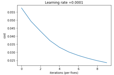

이번엔 train과 test acc를 확인해보자.

# Plot the train accuracy
plt.plot(np.squeeze(train_acc))
plt.ylabel('Train Accuracy')
plt.xlabel('iterations (per fives)')
plt.title("Learning rate =" + str(0.0001))
# Plot the test accuracy
plt.plot(np.squeeze(test_acc))
plt.ylabel('Test Accuracy')
plt.xlabel('iterations (per fives)')
plt.title("Learning rate =" + str(0.0001))
plt.show()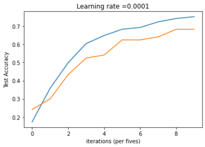

여기서 텐서플로우에 대한 설명을 마친다.