• parent: SqueezeLLM
• Settings
  • LLaMA, Llama-2, Llama-3, Mistral
  • Wikitext-2, C4
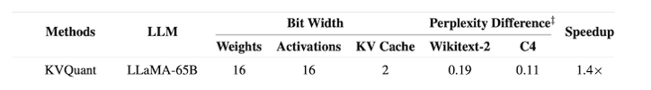
  • 1M on a single A100-80GB GPU, 10M on 8-GPU

Motivation

• small batch size에 대해서, LLM inference의 generation 단계는 memory bound함. (SqueezeLLM)

• memory bottleneck은 context size와 강한 연관이 있음.

• short sequence lengths: memory consumption의 주 요인 = weight matrix
  따라서, model size를 minimize해서, memory consumption과 bandwith requirement를 줄이는게 최선의 방법.

• 하지만, long sequence lengths: memory bottleneck의 주 요인 = Key와 Value를 Caching하기 위한 memory requirement.
  (batched inference를 고려한다면, 이 문제는 더욱 심각함.)

Background

LLM Inference

• small batch size에 대해서, LLM inference의 generation 단계는 memory-bandwidth bound하다.

• generation 동안, model은 이전에 generated된 output tokens에 condition generation하기 위해서,
  intermediate Key, Value activations를 store해야 한다.

• future tokens를 generation하기 위해, 각 prior token에 대해, 각 layer의 Keys와 Values를 store 해야 한다.

• 이 stored activations를 Key-Value(KV) cache라고 부른다.

• a model with

  • $n$ layers
  • $h$ attention heads with dimension $d$ that is stored using $e$ bytes per element,
  • KV cache size for batch size $b$ and sequence length $l$ is
    $2\cdot n \cdot h \cdot d \cdot e \cdot b \cdot l$
  • KV cache becomes the dominant contributor to memory consumption for longer sequence lengths and larger batch sizes.

• batch inference에서 각 sequence가 독립적인 KV 캐시를 필요로 함.
  이로 인해 memory bandwidth가 주요 bottleneck이 됨.
  따라서 KV Cache의 compression이 LLM의 성능 향상에 중요한 역할.

KV Cache Compression

• 이전 관련 연구들은 KV cache에서 중요한 token들만 store하고, 나머지 token들은 제거하는 방법들을 사용함.-

• 각 step마다 a subset of tokens를 retrieve해서 memory bandwidth를 줄이는 연구도 있음.

• KVQuant는 KV cache Quantization 방향으로 연구.

Methods

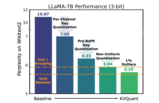
Per-Channel Key Quantization ➡️ Pre-RoPE Key Quantization ➡️ Non-Uniform KV Cache Quantization ➡️ Per-vector Dense-and-Sparse Quantization

1.Per-Channel Key Quantization

• KV Cache distribution

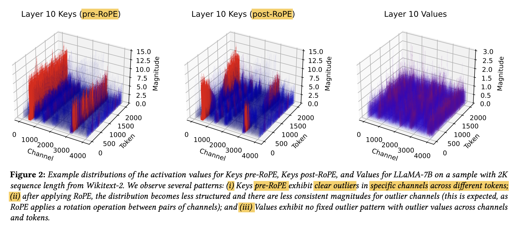
  • Key matrix들에서 distinct한 outlier channels를 가짐을 observe.
  • Value matrix들에선 outlier channels와 outlier tokens를 둘 다 가지며, Key 보다는 outlier magnitude가 작음을 observe.
  • 

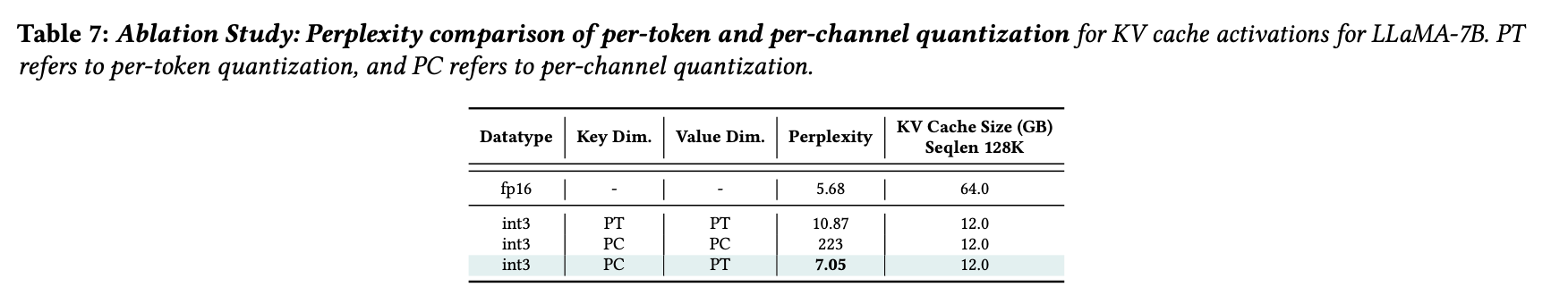
• 이전 KV cache Q 연구들은 "per-token quantization"

  • scaling factor, zero-point are shared by elements in the same token

• 이 연구에선, "per-channel KV cache Q"

  • scaling factor, zero-point are shared by elements in the same channel.

  • Keys에서는 효과적이지만, Values에서는 효과적 X를 발견 (Appendix E).

    • 따라서, Key는 per-chanel, Value는 per-token으로 Q
    • 

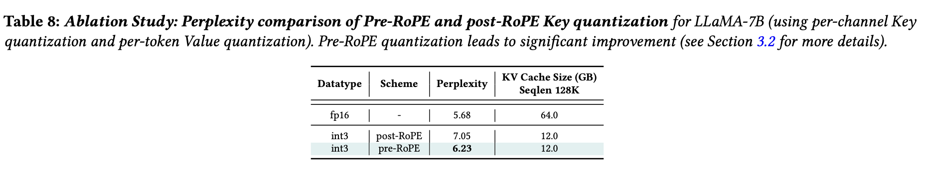
2. Pre-RoPE Key Quantization

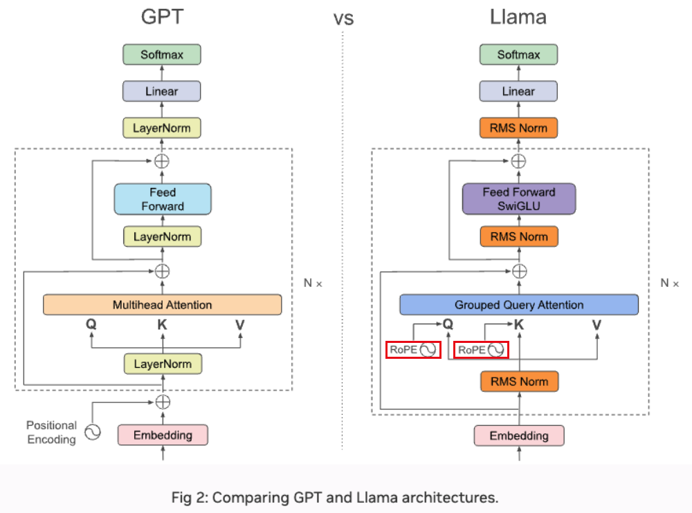
• Keys를 Q할 때 issue중 하나는, rotary positional embedding (RoPE)를 handling하는 것.

• RoPE는 대부분의 public LLMs에서, Keys와 Queries에 적용된다.

  • 

  • Query vector at position $m$, $Q_m = W_q * x_m$
    Key vector at position $n$, $K_n = W_k * x_n$ 이 주어질 때,

  • RoPE는 Query와 Key 벡터 사이의 relative position을 해당 position index의 배수에 해당하는 angle로 표현한다(embed).

  • RoPE는 self-attention에서 다음과 같이 적용된다.
    

• Key vector를 caching할 때, $\tilde{K}_n$을 cache하거나, (after applying RoPE)
  inference 도중에 on-the-fly로 $K_n$을 cache하고 $R^d_{\theta,n}$을 적용해야 한다. (before RoPE)

• RoPE 즉, rotation을 적용한 이후 key vectors를 caching 할 때의 challenge는
  sequence 내 서로 다른 position에 대해 channel 쌍들이 서로 다른 정도로 mix된다는 점이다.
  sequence 내 position에 따라 channel pair들이 서로 다른 angle로 함께 rotate되기 때문이다.

  • post-RoPE ativation distribution을 보면, channel pair들 간의 rotation이 channel magnitude의 일관성을 떨어뜨림(less consistent)을 볼 수 있다.
    
  • 이로 인해 일반적으로 일관된 큰 크기의 값을 갖는 Key activation channel을 Q하는 것이 더 어려워진다. (Motivation)

• 그래서, pre-RoPE Key Q를 하고, ($K_n$을 Q)
  deQ 이후에, on-the-fly로 positional embeddings를 적용하는 방법을 연구했다.
  (결과적으로, perplexity 향상됨)
  

• 참고: RoPE의 rotation matrix

  • 

3. nuqX: X-Bit Per-Layer Sensitivity-Weighted Non-Uniform Datatype

(🫶 SqueezeLLM)

• "각 layer에서 Q error에 대한 sensitivity를 분석하여,
  non-uniform Q의 quantization bins의 위치를 최적화하는 방법."

• non-uniform Q를 할거야.

  • Query와 Key activations는 non-uniform이잖아.

  • "overhead 문제 없어"
    KV cache loading은 memory bandwidth bound함
    (batch sizse 또는 sequence length에 상관없이),
    이는 non-uniform Q를 사용함으로써 발생되는 deQ overhead가 문제가 되지 않음을 뜻함.
    (더 computation 하는게 추가적인 latency를 발생시키진 않기 때문)

• "squeezeLLM가 sensitivity를 측정해서 non-uniform Q bins를 최적화하는 방법"을 따를건데, KV cache는 좀 다르게 해야함."

  • squeezeLLM
    • sensitivity-weighted k-means approach를 사용해 non-uniform quantization signposts를 compute함.
  • 하지만, 이 방법을 KV cache Q에 그대로 적용할 수 없음.
    • Values가 runtime에 online으로 quantized 되기 때문.
    • 즉, 우리가 inference 도중에 K-means를 적용해야 한다는 것인데,
      online으로 activation sensitivity를 estimation하는 것은 어려움.

• 따라서, "per-tensor non-uniform datatype" offline on calibration data를 도출해서,
  efiicient한 online non-uniform KV cache Q를 하겠어.

  • 이 data type은 key와 value distribution을 정확히 represent하도록, per-channel 또는 per-token으로 rescale됨.

• inference 이전에 calibration set에서 offline으로 sensitivity-weighted Q signposts를 계산

  • 이 때 shared datatype을 도출하기 전에, 각 channel을 별도로 [−1, 1] 범위로 정규화함으로써
    per-vector quantization과의 호환성을 유지

• "SqueezeLLM처럼, Fisher info matrix는 똑같이 사용할거야."
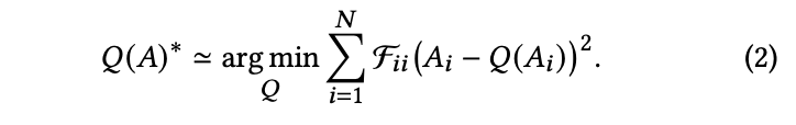
  Appendix B에서 유도된 대각 Fisher information matrix와 activation $A$에 대한 quantization error를 사용하여, 다음과 같이 error minimization objective를 공식화한다.

  • 

    • 여기서 A는 1차원으로 flattened되며, N은 calibration set의 모든 샘플에서 얻은 요소들의 수를 나타낸다.

    • 정규화된 activation 값들을 사용하여 적용할 수 있도록 Appendix C에 설명된 대로 Equation 2의 objective function을 수정.

    • 이후, calibration set에서 k-means solver를 사용하여 offline으로 이를 최소화함으로써,
      각 Key 또는 Value layer에 대한 non-uniform datatype의 quantization signposts를 얻음.

Fisher Information Matrix(FIM)가 모델의 민감도를 측정하는 원리

4.Per-Vector Dense-and-Sparse Q

(🫶 SqueezeLLM)

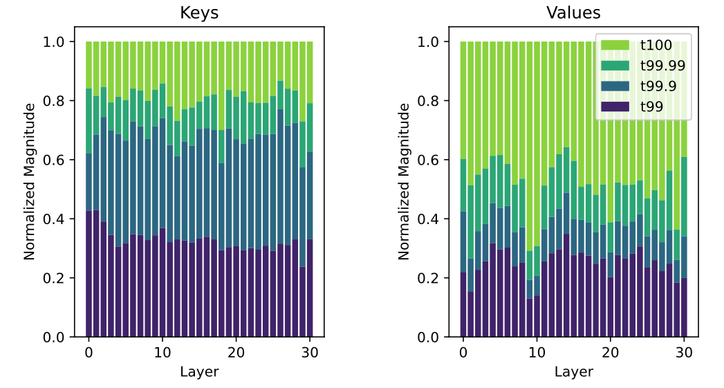
• Key와 Value activation들의 값 분포 ➡️ 대부분 집중되어 있고, 몇몇 outlier가 range를 넓힘.

  • 

  • t100, t99.99란?

    • t100: 모든 값들을 포함하는 전체 범위.
      즉, 최소값부터 최대값까지의 전체 dynamic range.
    • t99.99: 전체 값들 중 99.99%를 포함하는 범위.
      즉, 가장 극단적인 0.01%의 값들을 제외한 범위.

  • 해석

    • 대부분의 값들이 전체 dynamic range의 작은 부분에 집중되어 있음.

    • 예를 들어, t99 선은 전체 값들의 99%가 그 아래에 있음을 보여주며, 이는 극소수의 outlier 값들이 전체 dynamic range를 크게 확장시키고 있음을 의미.

    • 이러한 분석은 왜 dense-and-sparse approach가 효과적인지를 보여줌.
      소수의 outlier들을 별도로 처리함으로써, 대부분의 값들을 더 정확하게 표현할 수 있는 좁은 범위에 집중할 수 있음.

• SqueezeLLM처럼, dense-and-sparse quantization을 활용하여 소수의 numerical outlier들을 분리함으로써, 표현 범위를 제한하고, 나머지 요소들을 더 높은 정밀도로 표현할 수 있음.

  • 하지만 Key와 Value 분포를 보면, 서로 다른 channel과 token들이 각기 다른 평균 크기를 가지고 있음.
  • 
  • 따라서 한 channel에서는 outlier로 간주되는 요소가 다른 channel에서는 outlier가 아닐 수 있음.(해당 channel의 평균 크기가 더 클 수 있기 때문에).
  • 이로 인해 dense-and-sparse quantization을 단순히 적용하는 것은 최적의 결과를 내지 못할 수 있음.

• 따라서 range를 왜곡시키는 outlier 값들을 직접 타겟팅하는 것이 중요.

  • KVQuant는 per-vector dense-and-sparse quantization을 활용.

  • 각 layer마다 하나의 outlier threshold를 사용하는 대신,
    per-vector outlier threshold를 사용.

    • per-channel quantization의 경우 channel마다 별도의 threshold 사용
    • per-token quantization의 경우 token마다 별도의 threshold를 사용).

  • per-channel quantization for $\textcolor{red}{Keys}$,
    per-token quantization for $\textcolor{green}{Values}$,
    outperforms the standard per-token quantization approach for both Keys and Values. (Appendix E)
    

  • 상한과 하한의 outlier threshold를 결정한 후, 벡터에 남아있는 숫자들은 [−1, 1] 범위로 정규화.

  • 그 다음 Equation 2를 최소화(이때 outlier들은 무시(제거)).

  • 남은 숫자들에 대한 non-uniform datatype의 quantization signpost를 얻음.

• per-vector dense-and-sparse quantization을 위한 outlier threshold를 계산하는 것은 정확성과 효율성 측면에서 어려움을 가질 수 있음.

  • per-channel outlier threshold를 offline으로 정확하게 calibrate.
  • per-token outlier threshold는 online으로 효율적으로 계산할 수 있음을 보임. (Section 3.6에서)

5. Attention Sink-Aware Q

• 이전 연구에 따르면, LLM의 첫 몇 개 layer를 지난 후에는
  모델이 첫 번째 token에 큰 attention score를 할당하는 경향.

  • 첫 번째 token이 의미적으로(semantically) 중요하지 않은 경우에도 발생.
  • 모델이 첫 번째 token을 "sink"(흡수체)로 사용하는 경향이 있기 때문.

• Attention Sink 현상으로 인해 모델은 첫 번째 토큰의 quantization 오류에 불균형적으로 sensitive함.

  • 첫 번째 token만 fp16으로 유지함으로써 perplexity 개선을 얻을 수 있음. (특히 2-bit quantization에서 두드러짐.)
  • calibration 과정에서도 첫 번째 token을 fp16으로 유지.
    • nuqX datatype을 도출할 때 첫 번째 token 무시.
    • Key에 대한 scaling factor와 zero point를 offline으로 calibrate할 때도 첫 번째 token 무시.

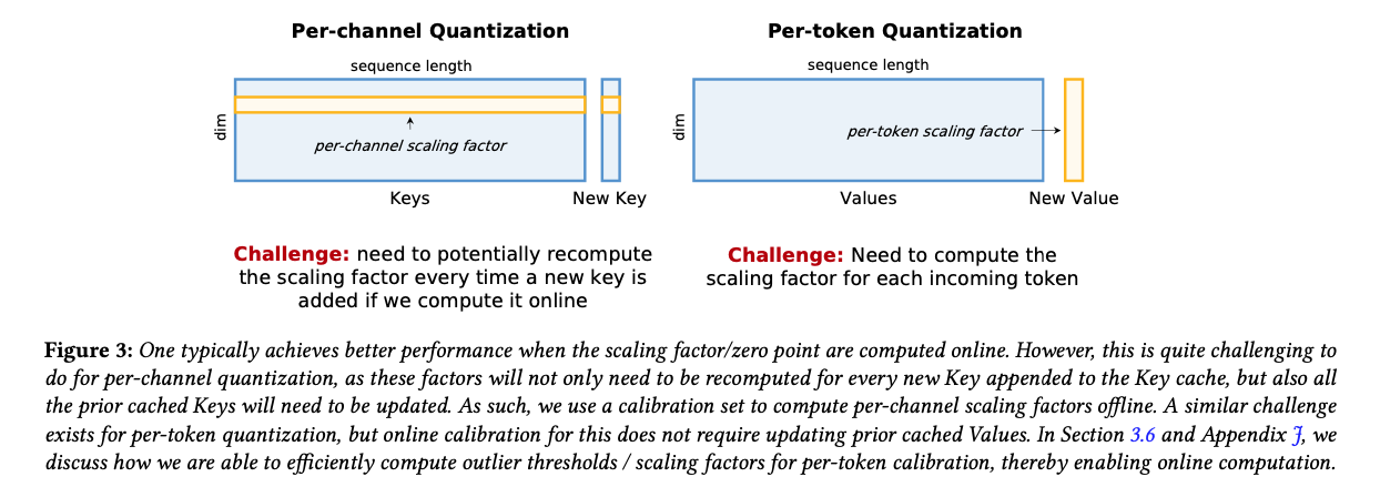
6. Offline Calibration vs Online Computation

• 

• activation quantization의 중요한 challenge

  • online computation: compute statistics on-the-fly (expensive)
  • offline computation: use offline calibration data
    (accuracy에 악영향)

• K: per-channel Q (for K) ➡️ Offline

  • scaling factor를 online으로 update하는 것은 어려움.

  • KV cache에 새로운 token이 추가될 때마다 각 incoming channel에 해당하는 scaling factor를 update 해야 함.

  • 따라서 statistics를 offline으로 계산.
    (즉, inference를 실행하기 전에 calibration 데이터를 사용하여 계산)

• V: per-token Q ➡️ Online

  • scaling factor를 offline으로 calibrate하는 것은 outlier Value token의 존재 때문에 어려움.
    (즉, 각 token마다 특성이 크게 다를 수 있어 offline calibration으로는 정확한 처리가 어렵다.)

  • 따라서 scaling factor와 outlier threshold를 online으로 계산.
    (각 incoming token에 대해 계산함.)

  • CPU로 offload하여 효율적으로 per-token outlier threshold를 online으로 계산 가능.(Appendix J)

Limitations

• 모델 훈련의 한계

  • 100K 이상의 긴 context length 모델 훈련에는 여전히 많은 작업이 필요함.
  • 본 연구는 긴 context length 모델의 효율적인 inference에 국한됨.

• Latency 벤치마킹의 한계

  • 현재 memory-bandwidth bound generation에 초점을 맞춤.
  • Prompt processing (여러 Key와 Value를 동시에 압축해야 하는 경우)에 대한 고려가 부족함.

• 현재 end-to-end 구현의 비효율성

  • Sparse matrix 업데이트를 위한 메모리 할당 처리에 비효율성 존재.
  • 이전 token의 데이터를 새 token의 데이터와 연결할 때 복사 작업 필요

• 향후 계획

  • Blocked allocation을 통해 메모리 재할당으로 인한 overhead 최소화.

---

Fisher Information Matrix(FIM)가 모델의 민감도를 측정하는 원리

1. Fisher Information의 정의

확률 변수 $X$가 파라미터 $\theta$를 가지는 확률 밀도 함수 $p(x \mid \theta)$를 따른다고 하자.
이때, Fisher Information Matrix $F(\theta)$는 log-likelihood 함수의 곡률을 기반으로 다음과 같이 정의된다:

또는 Hessian 형태로 표현하면,

여기서,

• $\log p(X \mid \theta)$ : log-likelihood 함수
• $\frac{\partial \log p(X \mid \theta)}{\partial \theta}$ : score function (점수 함수, likelihood의 기울기)
• $\mathbb{E}$ : $X$에 대한 기대값

FIM은 log-likelihood의 변화율의 변화율(즉, log-likelihood의 곡률)을 측정하는 값이다.

---

2. Fisher Information이 민감도를 측정하는 이유

2.1. Score Function의 역할

우선 score function을 정의하면,

이 함수는 파라미터 $\theta$에 대한 log-likelihood의 기울기를 나타내며, 특정 $\theta$에서 likelihood가 얼마나 빠르게 변하는지를 나타낸다.

• $S(\theta)$가 크면: 작은 변화에도 likelihood가 급격히 변하므로, 모델이 해당 파라미터에 매우 민감하다.
• $S(\theta)$가 작으면: likelihood가 완만하게 변하므로, 모델이 해당 파라미터 변화에 둔감하다.

따라서 $S(\theta)$의 분산이 클수록 모델이 해당 파라미터 변화에 민감함을 의미한다.

2.2. Fisher Information과 Score Function의 관계

FIM은 score function의 분산(즉, 2차 모멘트 기대값)으로 정의된다.

즉, FIM은 score function의 변동성을 측정하며, 파라미터 $\theta$가 변화할 때 모델의 출력이 얼마나 민감하게 반응하는지를 나타낸다.

• $F(\theta)$가 크면: 작은 변화에도 likelihood가 급격히 변하므로, 모델이 민감하게 반응한다.
• $F(\theta)$가 작으면: likelihood가 천천히 변하므로, 모델이 덜 민감하게 반응한다.

따라서 FIM은 모델이 특정 파라미터 변화에 대해 얼마나 "불확실성"을 가지는지 측정하는 척도이다.

---

3. 직관적인 해석

3.1. "정보량이 많을수록 작은 변화에도 큰 영향을 미친다"

FIM이 크다는 것은 log-likelihood의 변화가 크다는 의미이다. 즉, 파라미터가 살짝만 바뀌어도 확률 분포가 크게 변하는 경우이다.

예를 들어:

• 만약 카메라 초점이 맞춰진 사진이라면, 조금만 움직여도 초점이 흐려진다 (FIM 큼).
• 초점이 흐릿한 사진이라면, 조금 움직여도 별 차이가 없다 (FIM 작음).

즉, FIM이 크면 모델이 작은 변화에도 민감하게 반응하고, FIM이 작으면 모델이 무덤덤하게 반응한다.

---

3.2. "파라미터를 잘 추정할 수 있다면 모델이 민감한 것이다"

FIM이 크다는 것은 해당 파라미터를 더 정확하게 추정할 수 있다는 의미이기도 하다.
즉, 파라미터의 변화를 감지하기 쉽다는 뜻이며, 모델이 해당 파라미터에 민감하다는 의미이다.

예를 들어:

• 실험에서 어떤 변수를 조정했을 때 결과값이 크게 변하면 → 그 변수에 모델이 매우 민감함 (FIM 큼).
• 변수를 조정해도 결과가 거의 변하지 않으면 → 그 변수에 모델이 둔감함 (FIM 작음).

---

결론

• Fisher Information Matrix(FIM)는 likelihood 함수의 곡률을 측정하여, 모델이 특정 파라미터 변화에 얼마나 민감한지를 수학적으로 표현한다.
• Score function의 분산이 클수록 모델이 해당 파라미터에 대해 민감하게 반응한다는 의미.
• Cramér-Rao 하한을 통해, FIM이 클수록 파라미터를 더 정확하게 추정할 수 있으며, 이는 곧 해당 파라미터가 모델에서 중요한 역할을 한다는 것을 의미한다.