출처: Annotated Diffusion
내가 이해하기 위해 단순화한 버전
구현
신경망
bottleneck layer에서 가장 중요한 정보만 학습할 수 있는 U-Net 구조를 신경망으로 사용한다.
신경망은 특정 time step에서의 noised image를 입력받고, predicted noise를 반환해야 한다.
predicted noise는 input image와 동일한 size/resolution을 갖는 tensor임을 명심하자.
코드적으로, 신경망은 동일한 shape을 갖는 input과 output을 가진다.
이때 사용되는 신경망은 Autoencoder와 유사하다. Autoencoder는 encoder와 decoder 사이에 bottleneck layer를 갖는다.
encoder가 image를 bottleneck으로 불리는 작은 hidden representation으로 인코딩한다.
그리고 decoder는 이 hidden representation을 실제 image로 복원한다.
이 과정은 신경망이 bottleneck layer에서 가장 중요한 정보만 유지하도록한다.
DDPM 저자는 U-Net 구조를 사용했다.
U-Net은 여느 autoencoder와 같이, 신경망이 가장 중요한 정보만 학습할 수 있도록, 중간이 bottleneck으로 이루어져 있다.
중요한점은, U-Net은 encoder와 decoder 사이에 residual connection을 도입해서 gradient flow를 효과적으로 향상시켰다.
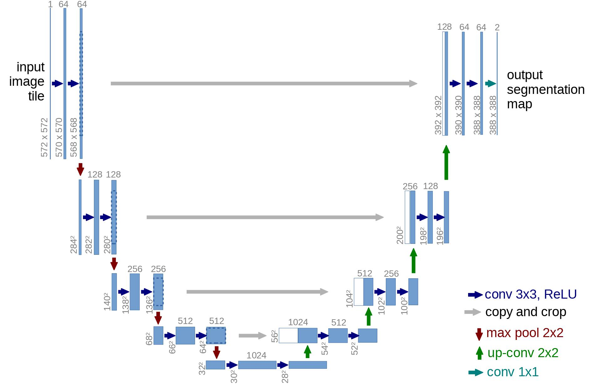
위 그림과 같이, U-Net model은 input을 downsampling하고, upsampling하는 방식으로 진행된다.
Network helpers
신경망 구현에 사용될 helper 함수와 클래스들을 먼저 정의한다.
def exists(x):
    return x is not None

def default(val, d):
    if exists(val):
        return val
    return d() if isfunction(d) else d


def num_to_groups(num, divisor):
    groups = num // divisor
    remainder = num % divisor
    arr = [divisor] * groups
    if remainder > 0:
        arr.append(remainder)
    return arr


class Residual(nn.Module):
    def __init__(self, fn):
        super().__init__()
        self.fn = fn

    def forward(self, x, *args, **kwargs):
        return self.fn(x, *args, **kwargs) + x


def Upsample(dim, dim_out=None):
    return nn.Sequential(
        nn.Upsample(scale_factor=2, mode="nearest"),
        nn.Conv2d(dim, default(dim_out, dim), 3, padding=1),
    )


def Downsample(dim, dim_out=None):
    # No More Strided Convolutions or Pooling
    return nn.Sequential(
        Rearrange("b c (h p1) (w p2) -> b (c p1 p2) h w", p1=2, p2=2),
        nn.Conv2d(dim * 4, default(dim_out, dim), 1),
    )
Position embeddings
신경망의 parameter가 time(noise level)간에 공유되기 때문에, 저자는 를 encoding하기 위해서, sinusoidal position embeddings를 사용했다.
(이 아이디어는 Transformer에서 비롯됐다.)
position embeddings는 신경망이 batch의 모든 이미지에 대해서,
어느 특정 time step(noise level)이 진행되고 있는지 "알도록" 한다.
SinusoidalPositionEmbeddings 모듈은
(batch_size, 1) shape의 tensor를 입력으로 받고
(i.e. batch 안의 여러 noisy image들의 noise levels),
(batch_size, dim) shape의 tensor를 출력한다.
여기서 dim은 position embeddings의 차원이다.
이 position embeddings는 각 residual block에 추가된다.
class SinusoidalPositionEmbeddings(nn.Module):
    def __init__(self, dim):
        super().__init__()
        self.dim = dim

    def forward(self, time):
        device = time.device
        half_dim = self.dim // 2
        embeddings = math.log(10000) / (half_dim - 1)
        embeddings = torch.exp(torch.arange(half_dim, device=device) * -embeddings)
        embeddings = time[:, None] * embeddings[None, :]
        embeddings = torch.cat((embeddings.sin(), embeddings.cos()), dim=-1)
        return embeddings
ResBet block
U-Net 모델의 핵심 building block을 정의한다.
DDPM 저자들은 Wide ResNet block을 사용하였지만,
Phil Wang이 "weight standardized" 버전의 standard convolution layer로 대체하였다.
이 대체한 버전이 group normalization과 조합했을 때 더 잘 동작한다.
class WeightStandardizedConv2d(nn.Conv2d):
    """
    https://arxiv.org/abs/1903.10520
    weight standardization purportedly works synergistically with group normalization
    """

    def forward(self, x):
        eps = 1e-5 if x.dtype == torch.float32 else 1e-3

        weight = self.weight
        mean = reduce(weight, "o ... -> o 1 1 1", "mean")
        var = reduce(weight, "o ... -> o 1 1 1", partial(torch.var, unbiased=False))
        normalized_weight = (weight - mean) / (var + eps).rsqrt()

        return F.conv2d(
            x,
            normalized_weight,
            self.bias,
            self.stride,
            self.padding,
            self.dilation,
            self.groups,
        )


class Block(nn.Module):
    def __init__(self, dim, dim_out, groups=8):
        super().__init__()
        self.proj = WeightStandardizedConv2d(dim, dim_out, 3, padding=1)
        self.norm = nn.GroupNorm(groups, dim_out)
        self.act = nn.SiLU()

    def forward(self, x, scale_shift=None):
        x = self.proj(x)
        x = self.norm(x)

        if exists(scale_shift):
            scale, shift = scale_shift
            x = x * (scale + 1) + shift

        x = self.act(x)
        return x


class ResnetBlock(nn.Module):
    """https://arxiv.org/abs/1512.03385"""

    def __init__(self, dim, dim_out, *, time_emb_dim=None, groups=8):
        super().__init__()
        self.mlp = (
            nn.Sequential(nn.SiLU(), nn.Linear(time_emb_dim, dim_out * 2))
            if exists(time_emb_dim)
            else None
        )

        self.block1 = Block(dim, dim_out, groups=groups)
        self.block2 = Block(dim_out, dim_out, groups=groups)
        self.res_conv = nn.Conv2d(dim, dim_out, 1) if dim != dim_out else nn.Identity()

    def forward(self, x, time_emb=None):
        scale_shift = None
        if exists(self.mlp) and exists(time_emb):
            time_emb = self.mlp(time_emb)
            time_emb = rearrange(time_emb, "b c -> b c 1 1")
            scale_shift = time_emb.chunk(2, dim=1)

        h = self.block1(x, scale_shift=scale_shift)
        h = self.block2(h)
        return h + self.res_conv(x)
Attention module
DDPM 저자들은 convolutional block들의 사이사이에 attention module을 추가했다.
Phil Wang는 2가지 방식의 attention을 사용했다.
첫 번째는 Transformer에서 사용된 보통의 multi-head self-attention이고,
두 번째는 linear attention variant 방식으로,
time과 memory requirements가 sequence length에 따라 linear하게 scale되는 방식이다.
(보통의 multi-head self-attention은 2차식을 따라 scale된다.)
class Attention(nn.Module):
    def __init__(self, dim, heads=4, dim_head=32):
        super().__init__()
        self.scale = dim_head**-0.5
        self.heads = heads
        hidden_dim = dim_head * heads
        self.to_qkv = nn.Conv2d(dim, hidden_dim * 3, 1, bias=False)
        self.to_out = nn.Conv2d(hidden_dim, dim, 1)

    def forward(self, x):
        b, c, h, w = x.shape
        qkv = self.to_qkv(x).chunk(3, dim=1)
        q, k, v = map(
            lambda t: rearrange(t, "b (h c) x y -> b h c (x y)", h=self.heads), qkv
        )
        q = q * self.scale

        sim = einsum("b h d i, b h d j -> b h i j", q, k)
        sim = sim - sim.amax(dim=-1, keepdim=True).detach()
        attn = sim.softmax(dim=-1)

        out = einsum("b h i j, b h d j -> b h i d", attn, v)
        out = rearrange(out, "b h (x y) d -> b (h d) x y", x=h, y=w)
        return self.to_out(out)

class LinearAttention(nn.Module):
    def __init__(self, dim, heads=4, dim_head=32):
        super().__init__()
        self.scale = dim_head**-0.5
        self.heads = heads
        hidden_dim = dim_head * heads
        self.to_qkv = nn.Conv2d(dim, hidden_dim * 3, 1, bias=False)

        self.to_out = nn.Sequential(nn.Conv2d(hidden_dim, dim, 1),
                                    nn.GroupNorm(1, dim))

    def forward(self, x):
        b, c, h, w = x.shape
        qkv = self.to_qkv(x).chunk(3, dim=1)
        q, k, v = map(
            lambda t: rearrange(t, "b (h c) x y -> b h c (x y)", h=self.heads), qkv
        )

        q = q.softmax(dim=-2)
        k = k.softmax(dim=-1)

        q = q * self.scale
        context = torch.einsum("b h d n, b h e n -> b h d e", k, v)

        out = torch.einsum("b h d e, b h d n -> b h e n", context, q)
        out = rearrange(out, "b h c (x y) -> b (h c) x y", h=self.heads, x=h, y=w)
        return self.to_out(out)
Group normalization
DDPM 저자들은 U-Net의 convolution/attenton layer에 group normalization을 추가했다.
아래 코드는 attention layer 이전에 group norm을 적용할 때 사용되는 PreNorm 클래스를 정의한다.
Conditional U-Net
이제 우리는 position embeddings, ResNet blocks, attention and group normalization과 같은 모든 building block들을 정의했고, 전체적인 신경망을 정의할 차례이다.
network 는 a batch of noised images와 각 noised image들의 time step(noise level)을 입력으로 받고,
image에 추가된 noise를 출력한다.
조금더 형식화해서 표현하면,
신경망은 입력으로
1)(batch_size, num_channels, height, width)shape의 a batch of noisiy images과
2)(batch_size, 1)shape의 noise level(=time step)을 입력받는다.
신경망은 출력으로
(batch_size, num_channels, heigh, width)shape의 added noise를 표현하는 tensor를 출력한다.
신경망은 다음 순서로 구성된다.
- convolution layer가 a batch of noisy images에 적용되고,
noise level(=time step)을 위한 position embeddings가 계산된다.- 일련의 downsampling 과정이 진행된다.
각 downsampling 단계는 2개의 ResNet block + groupnorm + attention + residual connection + a downsample opeartion 으로 구성된다.
(신경망의 중간에, ResNet block이 attention과 함께 다시 적용된다.)- 일련의 upsampling 과정이 진행된다.
각 upsampling 단계는 2개의 ResNet block + groupnorm + attention + residual connection + an upsample operation 으로 구성된다.- 마지막으로, convolutional layer과 ResNet block이 적용된다.
class Unet(nn.Module):
	def __init__(
    	self,
        dim,
        init_dim=None,
        out_dim=None,
        dim_mults=(1, 2, 4, 8),
        channels=3,
        self_condition=False,
        resnet_block_groups=4,
    ):
    	super().__init__()

        # determine dimensions
        self.channels = chaneels
        self.self_condition = self_condition
        input_channels = channels * (2 if self_condition else 1)

        init_dim = default(init_dim, dim)
        self.init_conv = nn.Conv2d(input_channels, init_dim, 1, padding=0) # changed

        dims = [init_dim, *map(lambda m: dim * m, dim_mults)]
        in_out = list(zip(dims[:-1], dims[1:]))

        block_klass = partial(ResnetBlock, groups=resnet_block_groups)

        # time embeddings
        time_dim = dim * 4

        self.time_mlp = nn.Sequential(
        	SinusoidalPositionEmbeddings(dim),
            nn.Linear(dim, time_dim),
            nn.GELU(),
            nn.Linear(time_dim, time_dim),
        )

        # layers
        self.downs = nn.ModuleList([])
        self.ups = nn.ModuleList([])
        num_resolutions = len(in_out)

        for ind, (dim_in, dim_out) in enumerate(in_out):
        	is_last = ind >= (num_resolutions - 1)

        	self.downs.append(
        		nn.ModuleList(
            		[
                		block_klass(dim_in, dim_in, time_emb_dim=time_dim),
	                    block_klass(dim_in, din_in, time_emb_dim=time_dim),
	                    Residual(PreNorm(dim_in, LinearAttention(dim_in))),
	                    Downsample(dim_in, dim_out)
    	                if not is_last
	                    else nn.Conv2d(dim_in, dim_out, 3, padding=1)
                	]
	            )
	        )

    	    mid_dim  = dims[-1]
            self.mid_blcok1 = block_klass(mid_dim, mid_dim, time_emb_dim=time_dim)
            self.mid_attn = Residual(PreNorm(mid_dim, Attention(mid_dim)))
            self.mid_block2 = block_klass(mid_dim, mid_dim, time_emb_dim=time_dim)

            for ind, (dim_in, dim_out) in enumerate(reversed(in_out)):
            	is_last = ind == (len(in_out - 1 )

                self.ups.append(
                	nn.ModuleList(
                    	[
                        	block_klass(dim_out + dim_in, dim_out, time_emb_dim=time_dim)
                            block_klass(dim_out + dim_in, dim_out, time_emb_dim=time_dim)
                            Residual(PreNorm(dim_out, LinearAttention(dim_out))),
                            Upsample(dim_out, dim_in)
                            if not is_last
                            else nn.Conv2d(dim_out, dim_in, 3, padding=1)
                        ]
                    )
                )

			self.out_dim = default(out_dim, channels)

            self.final_res_block = block_klass(dim*2, dim, time_emb_dim=time_dim)
            self.final_conv = nn.Conv2d(dim, self.out_dim, 1)

		def forward(self, x, time, x_self_cond=None):
        	if self.self_condition:
            	x_self_cond = default(x_self_cond, lambda: torch.zeros_like(x))
                x = torch.cat((x_self_cond, x), dim=1)

            x = self.init_conv(X)
            r = x.clone()

            t = self.time_mlp(time)

            h = []

            for block1, blokc2, attn, downsample in self.downs:
            	x = block1(x, t)
                h.append(x)

                x = block2(x, t)
                x = attn(x)
                h.append(x)

                x = downsample(x)

                x = downsample(x)

			x = self.mid_block1(x, t)
            x = self.mid_attn(x)
            x = self.mid_block2(x, t)

            for block1, block2, attn, upsample in self.ups:
            	x = torch.cat((x, h.pop()), dim=1)
                x = block1(x, t)

                x = torch.cat((x, h.pop(), dim=1)
                x = block2(x, t)
                x = attn(x)

                x = upsample(x)

        	x = torch.cat((x, r), dim=1)

            x = self.final_res_block(x, t)
            return self.final_conv(x)
Forward Diffusion Process 정의하기
forward process는 real distribution에서 뽑은 image에 점진적으로 noise를 추가한다. 이때, time steps 만큼 진행된다.
이 과정은 variance schedule에 따라 진행된다.
DDPM 저자들은 linear schedule을 사용했다.

하지만, 이후 논문에서 consie schedule을 사용했을 때 더 좋은 결과를 낼 수 있음이 밝혀졌다.
아래 코드는 time steps 동안 variance scheduling하는 코드이다.
def cosine_beta_schedule(timesteps, s=0.008):
    """
    cosine schedule as proposed in https://arxiv.org/abs/2102.09672
    """
    steps = timesteps + 1
    x = torch.linspace(0, timesteps, steps)
    alphas_cumprod = torch.cos(((x / timesteps) + s) / (1 + s) * torch.pi * 0.5) ** 2
    alphas_cumprod = alphas_cumprod / alphas_cumprod[0]
    betas = 1 - (alphas_cumprod[1:] / alphas_cumprod[:-1])
    return torch.clip(betas, 0.0001, 0.9999)

def linear_beta_schedule(timesteps):
    beta_start = 0.0001
    beta_end = 0.02
    return torch.linspace(beta_start, beta_end, timesteps)

def quadratic_beta_schedule(timesteps):
    beta_start = 0.0001
    beta_end = 0.02
    return torch.linspace(beta_start**0.5, beta_end**0.5, timesteps) ** 2

def sigmoid_beta_schedule(timesteps):
    beta_start = 0.0001
    beta_end = 0.02
    betas = torch.linspace(-6, 6, timesteps)
    return torch.sigmoid(betas) * (beta_end - beta_start) + beta_start
우선 time steps 동안 linear schedule을 사용하고,
cumulative product 연산 등에 필요한 부터 다양한 변수들을 정의해보자.
각 변수들은 1D tensor들이고, 부터 까지의 value들을 저장하고 있다.
중요한 부분으로, 우리는 extract 함수도 정의한다.
이 함수는 a batch of indices에서 적합한 를 뽑아내는데 사용된다.
timesteps = 300

# define beta schedule
betas = linear_beta_schedule(timestpes=timesteps)

# define alphas
alphas = 1. - betas
alphas_cumprod = torch.cumprod(alphas, axis=0)
alphas_cumprod_prev = F.pad(alphas_cumprod[:-1], (1,0), value=1.0)
sqrt_recip_alphas = torch.sqrt(1.0 / alphas)

# calculations for diffusion q(x_t | x_{t-1}) and others
sqrt_alphas_cumprod = torch.sqrt(alphas_cumprod)
sqrt_one_minus_alphas_cumprod = torch.sqrt(1. - alphas_cumprod)

# calculations for posterior q(x_{t-1} | x_t, x_0)
posterior_variance = betas * (1. - alphas_cumprod_prev) / (1. - alphas_cumprod)

def extract(a, t, x_shape):
	batch_size = t.shape[0]
    out = a.gather(-1, t.cpu())
    return out.reshape(batch_size, *((1,), * (len(x_shape) - 1)).to(t.device)
이제 고양이 이미지를 이용해서 diffusion process의 각 time step마다 어떻게 noise가 추가되는지 시각화해보자.
from PIL import Image
import requests

url = 'http://images.cocodataset.org/val2017/000000039769.jpg'
image = Image.open(requests.get(url, stream=True).raw) # PIL image of shape HWC
image
실제로 noise는 Pillow 이미지들에 추가되는 것이 아니라, PyTorch tensor에 추가된다.
따라서 PIL image를 PyTorch tensor로 변환하는 image transformation들을 정의하고,
역시 PyTorch tensor를 PIL image로 변환하는 image transformation들도 정의한다.
이 transformation 과정은 꽤 간단하다.
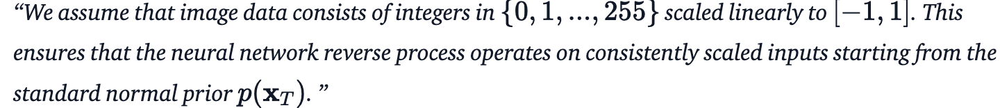
먼저 image를 255로 나누어 [0,1] 범위 안에 표현될 수 있도록 normalize한다.
그리고 이미지가 [-1, 1] 범위 안에 있도록 만들어준다.
DDPM 논문에는 다음과 같이 나와있다.
PIL image ➡️ Pytorch tensor
from torchvision.transfroms import Compose, ToTensor, Lambda, ToPILImage, CenterCrop, Resize

image_size = 128
transfrom = Compose([
	Resize(image_size),
    CenterCrop(image_size),
    ToTensor(), # turn into torch Tensor of shape CHW, divide by 255
    Lambda(lambda t: (t*2) - 1), # values in range [-1, 1]
])

x_start = transform(image).unsqueeze(0)
x_start.shape # torch.Size([1, 3, 128, 128])
Pytorch tensor ➡️ PIL image
[-1, 1] 사이의 값들을 포함하는 Pytorch tensor를 PIL image로 다시 변환하는 변환을 정의한다.
import numpy as np

reverse_transform = Compose([
	Lambda(lambda t: (t+1) / 2), # values range from [-1, 1] to [0, 1]
    Lambda(lambda t: t.permute(1, 2, 0)),
    Lambda(lambda t: t*255.), # values range from [0, 1] to [0, 255]
    Lambda(lambda t: t.numpy().astype(np.uint8)),
    ToPILImage(),
])
Forward Process
이제 forward diffusion process를 정의하자.

# forward diffusion
def q_sample(x_start, t, noise=None):
	if noise is None:
    	noise = torch.randn_like(x_start)

	sqrt_alphas_cumprod_t = extract(sqrt_alphas_cumprod, t, x_start.shape)
    sqrt_one_minus_alphas_cumprod_t = extract(
    	sqert_one_minus_alphas_cumprod, t, x_start.shape
    )

    return sqrt_alphas_cumpord_t * x_start + sqrt_one_minus_alphas_cumprod_t * noise
특정 time step에 대해서 test해보자
def get_noisy_image(x_start, t):
	# add noise
    x_noisy = q_sample(x_start, t=t)

    # turn back into PIL image
    noisy_image = reverse_transfrom(x_noisy.squeeze())

    return noisy_image


# take time step
t = torch.tensor([40])
get_noisy_image(x_start, t)
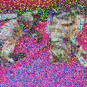
이번엔 더 다양한 time step의 결과를 시각화해보자.
import matplotlib.pyplot as plt

# use seed for reproducability
torch.manual_seed(0)

def plot(imgs, with_orig=False, row_title=None, **imshow_kwargs):
	if not isinstance(imgs[0], list):
    	# Make a 2 grid even if there's just 1 row
        imgs = [imgs]

    num_row = len(imgs)
    num_cols = len(imgs[0]) + with_orig
    fig, axs = plt.subplots(figsize=(200, 200), nrows=num_rows, ncols=num_cols, squeeze=False)
    for row_idx, row in enumerate(imgs):
    	row = [image] + row if with_orig else row
        for col_idx, img in enumerate(row):
        	ax = axs[row_idx, col_idx]
            ax.imshow(np.asarray(img), **imshow_kwargs)
            ax.set(xticklabels=[], yticklabels=[], xticks=[], yticks=[])

    if with_orig:
    	axs[0, 0].set(title='Original image')
        axs[0, 0].title.set_size(8)
    if row_title is not None:
	    for row_idx in range(num_rows):
        	axs[row_idx, 0].set(ylabel=row_title[row_idx])

    plt.tight_layout()

plot([get_noisy_image(x_start, torch.tensor([t])) for t in [0, 50, 100, 150, 199]])
Loss function
위 과정은 우리가 이제 loss function을 정의할 수 있음을 의미한다. 아래 코드에서 denoise_model은 우리가 정의한 U-Net 신경망이 될것이다.
def p_losses(denoise_model, x_start, t, noise=None, loss_type="l1"):
	if noise is None:
    	noise = torch.randn_like(x_start)

    # noised image
    x_noisy = q_sample(x_start=x_start, t=t, noise=noise)
    # predicted noise
    predicted_noise = denoise_model(x_noisy, t)

    if loss_type == 'l1':
    	loss = F.l1_loss(noise, predicted_noise)
	elif loss_type == 'l2':
    	loss = F.mse_loss(noise, predicted_noise)
	elif loss_type == "huber":
    	loss = F.smooth_l1_loss(noise, predicted_noise)

	return loss
PyTorch Dataset + DataLoader 정의하기
여기서 우리는 보통의 PyTorch Dataset을 정의한다.
Fasho-MNIST, CIFAR-10 또는 ImageNet과 같은 real dataset으로 구성되어 있고, [-1,1]로 linearly scaled 되어 있다.
각 image는 동일한 크기로 resize 되어있다.
그리고 논문에서처럼 random하게 horizontally flipped 되어있다.

여기에서는 Fashion MNIST dataset을 쉽게 load해서 사용한다.
이 데이터셋은 동일한 resolution 28x28을 갖진 이미지들로 구성되어 있다.
from datasets import load_dataset

# load dataset from the hub
dataset = load_dataset("fashion_mnist")
image_size = 28
channels = 1
batch_size = 128
그 다음 모든 데이터셋에 적용할 기본적인 image processing 함수를 정의한다. 이때 dataset library의 with_transform 기능을 사용했다.
image processing에는 random horizontal flips, rescaling 그리고 최종적으로 [-1, 1] 범위의 값을 갖도록 하는 연산이 포함돼있다.
from torchvision import transforms
from torch.utils.data import DataLoader

# define image transformations
transform = Compose([
	transforms.RandomHorizontalFlip(),
    transforms.ToTensor(),
    transforms.Lambda(lambda t: (t*2) - 1)
])

# define function
def transforms(examples):
	examples["pixel_values"] = [transform(image.convert("L")) for image in examples["image"]]
    del examples["image"]

    return examples

transformed_dataset = dataset.with_transform(transforms).remove_columns("label")

# create dataloader
dataloader = DataLoader(transformed_dataset["train"], batch_size=batch_size, shuffle=True)

batch = next(iter(dataloader))
print(batch.keys()) # dict_keys(['pixel_values'])
Sampling
progress를 tracking 하기 위해서, model을 training하는 동안에 sampling 하기 위한 코드를 정의한다.
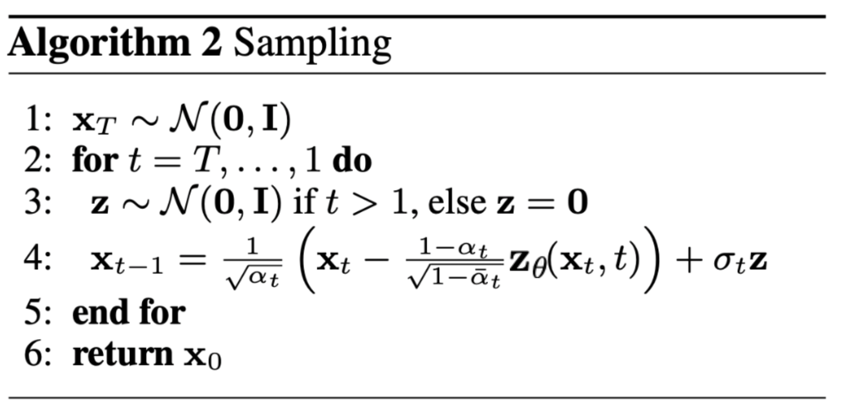
diffusion model에서 새로운 image 생성은 reverse processs를 통해 이루어진다.
1) time step 의 pure noise에서 Gaussian distribution을 sampling한다.
2) time step 부터 까지, 신경망을 사용해서, 신경망이 학습한 conditional probability를 이용해 점진적으로 denoise한다.
위 에서 볼 수 있듯, mean을reparameterization하여 만든 우리의 noise predictor를 이용해서,
우리는 조금 더 적게 denoise된 image 을 얻을 수 있다.
(참고로, DDPM에서 분산은 고정된 값으로 known value이다)
이 과정을 통해 real data distribution 에서 생성된 것과 유사한 새로운 image를 얻게된다.
@torch.no_grad()
def p_sample(model, x, t, t_index):
	betas_t = extract(betas, t, x.shape)
    sqrt_one_minus_alphas_cumprod_t = extract(
    	sqrt_one_minus_alphas_cumprod, t, x.shape
    )
    sqrt_recip_alphas_t = extract(sqrt_recip_alphas, t, x.shape)

    # Equation 11 in the paper
    # Use our model (noise predictor) to predict the mean
    model_mean = sqrt_recip_alphas_t * (
    	x - betas_t * model(x, t) / sqrt_one_minus_alphas_cumprod_t
    )

    if t_index == 0:
    	return model_mean
	else:
    	posterior_variance_t = extract(
        	posterior_variance, t, x.shape
        )
        noise = torch.randn_like(x)
        # Algorithm2 line 4:
        return model_mean + torch.sqrt(posterior_variance_t) * noise

# Algorithm 2 (includint returning all images)
@torch.no_grad()
def p_sample_loop(model, shape):
	device = next(model.parameters()).device

    b = shape[0]
    # start from pure noise (for each example in the batch)
    img = torch.randn(shape, device=device)
    imgs = []

    for i in tqdm(reversed(range(0, timesteps)), desc = 'sampling loop time step', total=timesteps):
    	img = p_sample(model, img, torch.full((b,), i, device=device, dtype=torch.long), i)
    	imgs.append(img.cpu().numpy())
	return imgs

@torch.no_grad()
def sample(model, image_size, batch_size=16, channels=3):
	return p_sample_loop(model, shape=(batch_size, channels, image_size, image_size))
Train the Model
생성된 이미지를 저장하기 위한 로직
from pathlib import Path

def num_to_groups(num, divisor):
	groups = num // divisor
    remanider = num & divisor
    arr = [divisor] * groups
    if remainder > 0:
    	arr.append(remainder)
	return arr

results_folder = Path("./results")
results_folder.mkdir(exist_ok=True)
save_and_sample_every = 1000
아래 코드는 model을 정의하고, GPU로 옮긴다.
opimizer도 정의한다.
from torch.optim import Adam

device = "cuda" if torch.cuda.is_available() else "cpu"

model = Unet(
	dim=image_size,
    channels=channels,
    dim_mults=(1, 2, 4,)
)
model.to(device)

optimizer = Adam(model.parameters(), lr=1e-3)
training을 시작해보자!
from torchvision.utils import save_image

epochs = 6

for epoch in range(epochs):
	for step, batch in enumerate(dataloader):
    	optimizer.zero_grad()

        batch_size = batch["pixel_values"].shape[0]
        batch = batch["pixel_values"].to(device)

        # Algorithm 1 line 3: sample t uniformally for every example in the batch
        t = torch.randint(0, timesteps, (batch_size,), device=device).long()

		loss = p_losses(denoise_model=model, x_start=batch, t=t, loss_type="huber")

        if step % 100 == 0:
        	print("Loss:", loss.item())

        loss.backward()
        optimizer.step()

        # save generated images
        if step != 0 and step % save_and_sample_every == 0:
        	milestone = step // save_and_sample_every
            batches = num_to_groups(num=4, divisor=batch_size)
            all_images_list = list(map(lambda n: sample(model, batch_size=n, channels=channels), batches))
            all_images = torch.cat(all_images_list, dim=0)
            all_images = (all_images+1) * 0.5 # [-1, 1] 범위를 갖는 이미지를 [0, 1] 범위로 정규화
            save_image(all_images, str(results_folder / f'smaple-{milestone}.png'), nrow=6)
Sampling (Inference)
model로부터 sampling하기 위해, 우리가 위에 정의한 sample 함수를 사용하면 된다.
# sample 64 images
samples = sample(model, image_size=image_size, batch_size=64, channels=channels)

# show a random one
random_index = 53
plt.imshow(samples[-1][random_index].reshape(image_size, image_size, channels), cmap="gray")
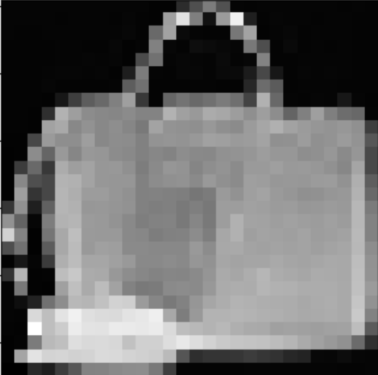
model이 handbag 이미지를 잘 생성하는 것 같다.
우리가 학습에 사용한 데이터셋은 꽤 낮은 해상도를 갖는(28x28) 이미지임을 고려하자.
denoising process를 gif로 만들 수 있다.
import matplotlib.animation as animation

random_index = 53

fig = plt.figure()
ims = []
for i in range(timesteps):
	im = plt.imshow(samples[i][random_index].reshape(image_size, image_size, channels), cmap="gray", animated=True)
    ims.append([im])

animate = animation.ArtistAnimation(fig, ims, interval=50, blit=True, repeat_delay=1000)
animate.save('diffusion.gif')
plt.show()
안녕하세요.
정말 도움 많이 되었습니다. 감사합니다.
질문 하나 드려도 될까요?
ViT 논문에서는 attention 적용시, feature map 내의 위치가 중요해서
명시적으로 positional embedding을 적용했는데,
위 UNet 구조에서는 time은 embedding 했지만,
feature map 내의 위치가 embedding 되는 부분이 없는 것 같아요.
혹시, 그 이유를 알 수 있을까요?
감사합니다.