[DETR] End-to-End Object Detection with Transformers (ECCV 2020)

YEOM JINSEOP·2023년 9월 27일

[3D Vision] Transformer based 3DSS

목록 보기

4/5

Authors: Nicolas Carion, Francisco Massa, Gabriel Synnaeve, Nicolas Usunier, Alexander Kirillov, and Sergey Zagoruyko

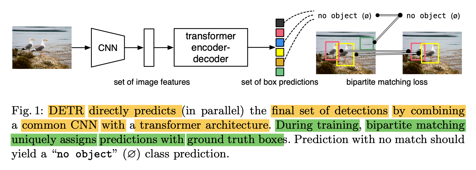
DETR is a new method
that views object detection
as a "direct set prediction problem".
,
predicts all objects at once.
Removes the need for
many hand-designed components
like a 'non-maximum suppression procedure' or 'anchor generation'
that explictly encoder our prior knowledge
about the task

🔑 Key Points

Main ingredients of DETR,
1) Set-based global loss ("a set loss function")
that forces unique predictions
via bipartite matching
between predicted & GT objects

➕

2) Transformer encoder-decoder architecture
with (non-autoregressive) parallel decoding"
that predidcts a set of objects & models their relation.

(Self-Attention mechainsm,
which explicitly model all pairwise interactions
between elements in a sequence,
make suitable for
constraints of set predictions
such as removing duplicate predictions)
Given a fixed small set of "learned object queries",
DETR reasons about
1) Relations of the objects
2) Global image context
to directly output the final set of predictions
in parallel.

1) Set Prediction Loss

1-1) Object Detection Set Prediction Loss

DETR infers a fixed-size set of $N$ predictions,
in a single pass
through the decoder
(where $N$ is set to be
significantly larger than
the number of objects in an image)
Main difficulty of training is
to score Predicted objects (class, position, size)
w.r.t. Ground Truth.
1) Our loss produces
an optimal Bipartite matching
between predicted & GT objects.
2) And then, optimize object-specific (bounding box) losses.

STEP 1) Bipartite Matching

To find Bipartite Matching
between Predicted & GT set of objects,
➡️ we search for a permutation of $N$ elements $\sigma$
with the lowest cost.

$y$ : GT set of objects,
$\hat{y}$ Prediction set of objects $(\in \{\hat{y}_i\}^N _{i=1})$ ,
$σ(i)$ : index $i$ ,
$L_{match}(y_i, \hat{y}_{σ(i)})$ : pair-wise matching cost
between $y_i$ and $\hat{y}_{σ(i)}$

(Assuming $N$ is larger than
the number of objects in the image,
we consider $y$ also as a set of size $N$
padded with $\emptyset$ (no object)).
This optimal assignment is computed efficiently
with the Hungarian algorithm,
following prior work.

Detail

Each element $i$ of the GT set
can be seen as a $y_i = (c_i, b_i)$

$c_i$ : target class label (which may be $\emptyset$ )
$b_i$ $\in$ $[0, 1]^4$ : vector that defines
GT box center coordinates, height, width
relative to image size.
Each element of the Prediction set, with index $σ(i)$
$c_i$ : probabiliry of class (as $\hat{y}_{σ(i)} (c_i)$ )
$\hat{b_σ(i)}$ : predicted box.
we define $L_{match} (y_i, \hat{y}_σ(i))$ :
This procedure of finding matching
plays the same role as
the heuristic assignment rules
used to match proposal or anchors to GT obejcts
in modern detectors.
'
main difference: we need to find one-to-one matching
for direct set prediction w.o duplicates

STEP 2) Optimize Object-Specific Loss

To compute loss function, $Hungarian$ $Loss$ for all pairs
mathced in previous step.
we define the loss
similarly to the losses of common object detectors,
(i.e., a linear combination of a negative log-likelihood
for class prediction and a box loss defined later):

$\hat{σ}$ : optimal assignment
computed in the 'First-Step'
(refer to paper for details )

Bounding box loss

Second part of the matching cost & Hungarian loss
is Bounding box loss $L_{box}(\cdot)$
that scores the bounding boxes.
Unlike many detectors that
do box predictions
as a w.r.t some initial guesses,
we make box predictions directly.
$L_box(b_i, \hat{b}_{σ(i)})$ :
(refer to paper for details )

⭐ 2) Transformer-based DETR Architecture

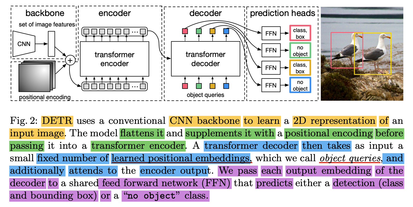
Three main components
1) a CNN backbone
to extract a compact feature representation
2) an encoder-decoder Transformer
3) a FFN(feed forward network)
that makes the final detection prediction.

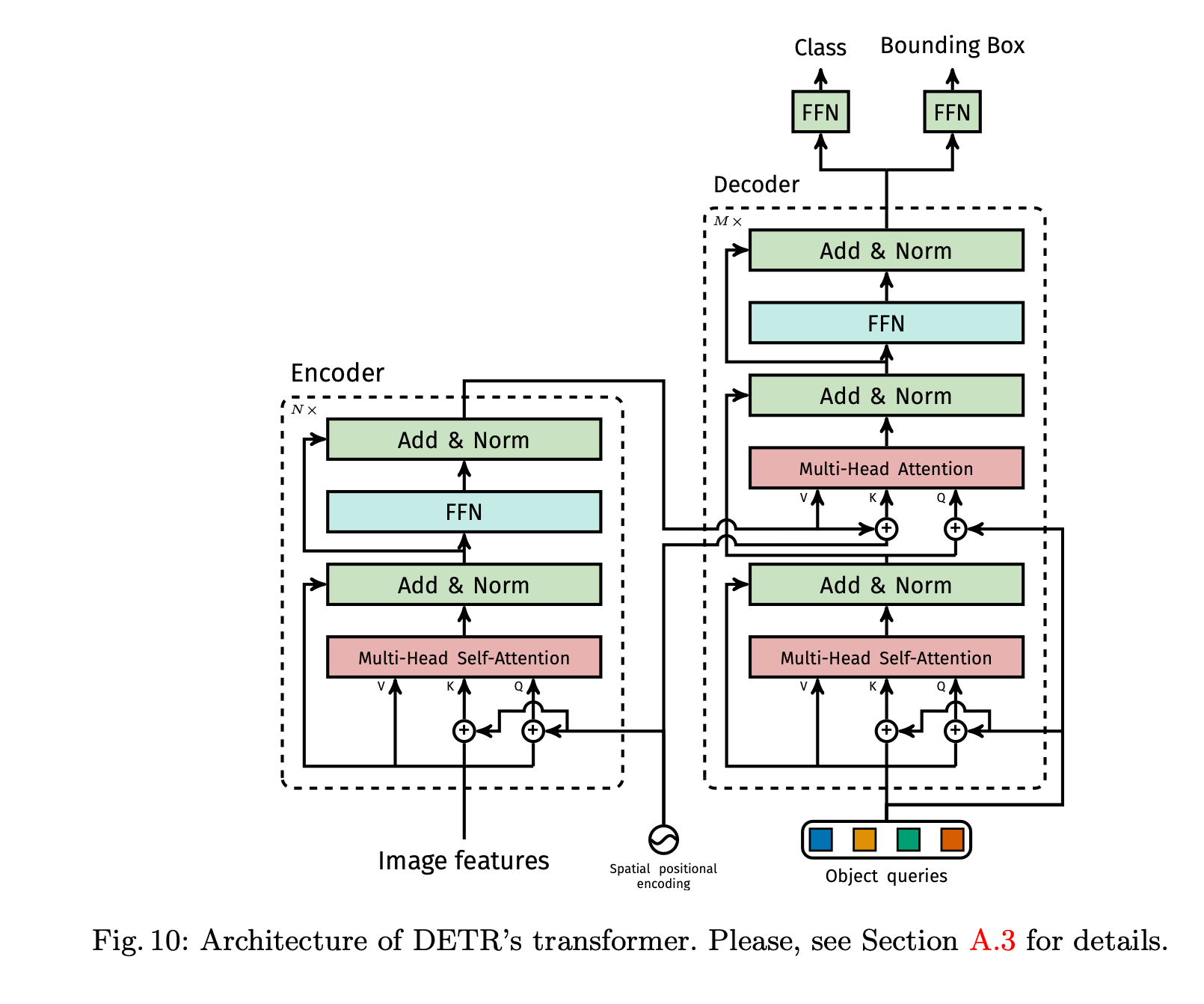
-----Encoder-----
feature map $f$ ➡️ smaller dimension feature map $z_0$ ➡️ one dimension feature map

-----Decoder-----
➡️ Object Queries ➡️ output embedding

-----FFN-----
➡️ ' bounding box coord.' & 'class labels' ➡️ resulting in final predictions

CNN Backbone

input: initial image $x_{img}$
$\in \mathbb{R}^{3 \times H_0 \times W_0}$ (with 3 color channels)
output: a lower-resolution feature map $f$
$\in \mathbb{R}^{C \times H \times W}$
(Typical values we use are
$C = 2048$ and $H, W = H_0 / 32, W_0 /32$ )

Transformer Encoder

feature map $f$ ➡️ smaller dimension feature map $z_0$ ➡️ one dimension feature map
First, 1 x 1 convolution
reduces the channel dimension of
high-level feature map $f$
from $C$ to a smaller dimension $d$ .

creating a new feature map $z_0$ ( $\in \mathbb{R}^{d \times H \times W}$ )
Encoder expects a sequence as input,
hence we collpase the spatial dimension of $z_0$
into one dimension,
resulting in a $d \times H W$ feature map
Each encoder layer has a standard architecture
consists of 'multi-head self-attention module' and a 'FFN'.
Fixed 'positional encodings' are added to
input of each attention layer,
Since transofrmer architecture is permutation-invariant

Transformer Decoder

Input: object queries(input embedding)
Output: output embedding

⭐ Object Query

Object Query는 Object Query Feature와 Object Query Positional Emedding으로 구성됨.

Object Query Feature는 Decoder에서 initial input으로 사용되어,
decoder layer를 거치면서 학습됨.
학습 시작 시 0으로 초기화 (zero-initialized)되며,
q

Object Query Positional Emedding은 Decoder Layer에서 attention 연산 시 모든 Query Feature에 더해짐.
학습 가능(learnable)함.

이러한 Object Qeury는 길이가 $N$ 으로,
Decoder에 의해 output embedding으로 변환(transform) 되며,
이후 FFN을 통해 각각 $independently$ 하게 box coordinate와 class label로 decode됨.
각각의 Object Query는 하나의 Object를 예측하는 region proposal에 대응된다고 볼 수 있다.
( $N$ 개의 Object를 예측하기 위한 일종의 Prior Knowledge로 볼 수 있음)
Object Query를 각 attention layer의 입력에 더해줌.
이때, embedding은 self-attention과 encoder-decoder attention을 통해
image 내의 전체 context에 대한 정보를 사용함.
이를 통해 object 사이의 pair-wise relation을 포착하여,
object간의 global한 정보를 모델링하는 것이 가능해짐.

Decoder follows the standard architecture of transformer,
transforming $N$ embeddings of size $d$
using multi-headed self- & encoder-decoder attention mechanisms,
Difference with the original transformer is that
our model decodes the $N$ objects in parallel
at each decoder layer.
(We refer the reader unfamiliar with the concepts to the suppl. materials)

Since the decoder is also 'permutation-invariant',
the $N$ "input embeddings" must be different to produce different results.
These "input embeddings" are learnt positional encodings
that we refer to as object queries,

and similarly to the encoder,
we add them to the input of each attention layer.
$N$ object queries are transformed into an "output embedding"
by the decoder.
They are then $independently$ decoded into 'box coordinates' and 'class labels'
by a FFN (described in the next).
resulting $N$ final predictions.
Using self- & encoder-decoder attention over these embeddings,
the model globally reasons about all objects together
using pair-wise relations between them,
while being able to use the whole image as context.

Prediction FFN (Feed-Forward Networks)

Decoder에서 출력한 output embedding을
3개의 linear layer와 ReLU activation function으로 구성된 FFN에 입력하여 최종 예측을 수행합니다.
FFN은 이미지에 대한 class label과 bounding box에 좌표(normalized center coordinate, width, height)를 예측합니다.
이 때 예측하는 class label 중 ∅은 객체가 포착되지 않은 경우로, "background" class를 의미합니다.

-----FFN-----
➡️ ' bounding box coord.' & 'class labels' ➡️ resulting in final predictions

Final prediction is computed by a 3-layer perceptron
with $ReLU$ ativation function & hidden dimension $d$ & a liner projection layer.
FFN predicts 'the normalized center coordinates', 'height & width of the box'
w.r.t the input image,
and Linear Layer predicts 'class label'
using a softmax function.
additional class label $\emptyset$
Since we predict a fixed-size set of $N$ bounding boxes,
(where $N$ is usually much larger than the actual number of objects of interest in an image,)
an additional class label $\emptyset$ is used to represent
that no object is detected within a slot.

This class plays a similar role to the "background" class
in the standard object detection approaches.

Auxiliary decoding losses

We found helpful to use 'auxiliary losses'
in decoder during training,
especially to help the model output
the correct number of objects of each class.
We add prediction FFNs & Hungarian loss
after each decoder layer.
All predictions FFNs share their parameters.
We use an additional shared layer-norm
to normalize the input to the prediction FFNs
from different decoder layers.