Abstract

• denoising diffusion model들의 생성 process는 굉장히 느린데,
  이는 번거로운 신경망에 의존하는, 긴 iterative noise estimation 때문이다.

  • 이 때문에 edge device들에 널리 사용되지 못하는 단점이 있다.

• 이전의 연구들은 diffusion 모델의 생성 과정을 가속화하기 위해, 효율은 많이 떨어트리지 않으면서도 더 짧은 sampling trajectory를 찾았다.

  • 하지만, 그 연구들은 무거운 신경망 안의 각 iteration에서의 비싼 noise estimation을 간과했다.

• 본 연구에서는, noise estimation network를 압축(compress)하는 관점으로 생성을 가속화한다.

  • diffusion model은 retraining에 어려움이 있기에,
    본 연구에서는 training-aware compression 패러다임은 제외했고,
    PTQ(post training quantization)을 diffusion model에 도입했다.

  • 하지만, noise estimation netowkrs의 output distribution이 time-step에 따라 변화하기 때문에,
    이전의 PTQ methods를 diffusion model에 적용하는 것은 실패한다.
    왜냐하면, single-time step 시나리오에 맞게 디자인되었기 때문이다.

  • diffusion model-specific한 PTQ method를 고안하기 위해,
    PTQ on DM을 세 가지 관점으로 연구했다.
    1) quantization operations,
    2) calibration dataset,
    3) calibration metric

  • 본 연구는 all-inclusive investigation으로부터의 여러 발견을 사용하고 요약했으며,
    이를 통해 본 연구를 수식화 했다.
    이 수식은 diffusion model의 unique한 multi-time-step 구조를 타겟으로 한다.

• 실험적으로, 본 연구의 method는 training-free manner로 성능을 유지하거나 심지어는 향상시키키면서도,
  full-precision diffusion model을 8-bit 모델로 direct하게 quantize할 수 있다.
  $\\$
  또한 중요하게, 우리 method는 예를 들어 DDIM과 같은 fast-sampling methods에 plug-and-play module 역할을 수행할 수 있다.

Introduction

연구 동향

• denoising process는 신경망을 통해 수천번의 timesteps로 noise estimation을 반복해야 한다.
  따라서, 생성 과정을 가속화하는것은 최근 활발한 연구 분야이다.
  4
  29
  24
  40
  2
  18

• diffusion model들을 가속화하기 위해서, 여러 접근들이 연구되고 있다.
  주로, 더 빠른 samplig strategy를 위해 trajectory를 sampling 하는 데 집중되어 있다.
  예를 들어,

  • 4
    29
    는 quality와 metrics를 좋게 유지하는 더 빠른 step size schedules를 제안했다.

  • 37
    은 denoising process에서 implicit phases를 적용했다

  • 2와 18은 생성 과정을 단순화하기 위해서 analytical approximations를 derive했다.

본 연구의 차별성

• 본 연구는 denoising process를 느리게 만드는 두 가지 orthgonal factors를 제안한다.
  1) noise로부터 image를 sampling 하기 위한 iterations
  2) 각 iteration에서 noise를 예측하기 위한 신경망

  • 기존 diffusion model 가속화 연구들은 주로
    1)에 집중하고, 2)는 간과하는 경향이 있다.
    4
    29
    24
    40
    2
    18
    $\\$
    
  • 신경망 compression 관점에서, 많은 network quantizastion과 pruning 연구들은 다음의 간단한 파이프라인을 따른다
    : original model을 training하고,
    quantized/pruned compressed model을 fine-tuning한다.
    17
    31
    $\\$
    
  • 특히, training-aware compression 파이프라인은 full training dataset을 요구하고
    end-to-end back-propagation을 수행하기 위해 많은 computation resource가 필요하다.
    $\\$
    

Diffusion에는 PTQ가 적합하다

• 하지만, diffusion model들은 아래 두 가지 이유로 training-aware compression이 적합하지 않다.

  • 1) training data가 privacy와 commercial 문제로 언제나 ready-to-use가 아니다.
    $\\$

  • 2) training process가 정말 expensive하다.
    예를 들어, DallE2나 ImageGen 같은 text-to-image model들을 위한 training data는 접근이 불가능하다.
    만약 접근이 가능하더라도, 그 데이터들을 fine-tuning하는 것은 수백 수천 GPU 시간이 소요될 것이다.
    $\\$

• Training-free network compression 기술이 diffusion model 가속을 위해 필요한 것이다.
  따라서, PTQ를 diffusion model 가속에 도입했다.
  22
  3
  17
  PTQ 방식으로 denoising 과정의 computation 속도를 높이고,
  diffusion 모델의 weight을 저장하기 위한 자원을 줄일 수 있다.

• PTQ는 장점이 많지만, diffusion model 안에서의 구현은 challenging하다.

  • 왜냐하면, diffusion 모델의 구조는 이전의 PTQ로 구현된 구조(예를 들어 image recognition을 위한 CNN, ViT)와는 굉장히 다르기 때문이다.
    $\\$
    특히, noise estimation network의 output distributions는 time-step에 따라 변화하기 때문에,
    single-time-step 시나리오로 고안된 이전 연구들의 PTQ 방식을 diffusion 모델에 적용하기 힘들다.

PTQ와 Diffusion Model 분석

• 본 연구는 다음 근본적인 질문에 답하려고 시도한다.
  : diffusion model process를 위한 PTQ의 core ingredients 설계(e.g. quantized operation selection, calibrations set collection, and calibration metric)는
  얼마나 quantized diffuion models의 성능에 영향을 미치는가?

  • 본 연구에서는 PTQ와 diffusion model을 각각, 그리고 연관지어서 분석한다.
  • 단순히 이전의 PTQ methods들을 일반화시켜서 diffusion model에 적용하는 것은 매우 큰 성능 하락을 불러일으킨다.
    denoising process에서 time-step에 따른 output distribution 차이가 크기 때문이다.
    $\\$
    다시 말하면, noise estimation network는 time-step에 의존한다.
    그리고 이 time-step에 따라 output distribution이 변화하는 것이다.
    $\\$
    이는 이전 연구들의 PTQ calibration의 핵심 모듈을 바로 사용할 수 없다는 것을 뜻한다.
    $\\$

Diffusion Model Specific Calibration Method

• 위의 관찰 결과를 바탕으로,
  diffusion model specific한 calibration method인
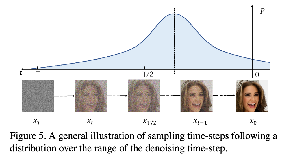
  NDTC(Normally Distributed Time-step Calibration)를 고안했다.

  이 방법은 skew normal distribution으로부터 a set of time-steps를 먼저 sampling하고,
  denoising process를 통해 sampled time-steps에 관해서 calibration samples를 생성한다.

• 이 방식으로, calibration set 안에서의 time-step 차이가 보완되고,
  PTQ4DM의 성능을 향상시킨다.

정리

• 본 연구에서는 diffusion model 가속화 방법인
  PTQ4DM(Post-Training for Diffusion Models)를 제안한다.

• 본 논문의 contributions는 다음 세 가지다.

  • 1) noise estimation networks가 direct하게 quantized되는
    PTQ를 도입한 diffusion model 가속화
    ( training-free network compression 관점에서의 첫 번째 diffusion model 가속화 연구 )
    $\\$

  • 2) 본 연구의 관찰 결과,
    다양한 time-setps에서의 output distribution은 diffusion model에 PTQ를 적용했을 때 큰 성능 하락을 일으킴.
    이 관찰 결과를 토대로, PTQ를 다른 관점에서 제안함
    $\\$

  • 3) 큰 성능 감소 없이 pre-trained diffusion model들을 8-bit로 quantize 가능함.
    plug-ang-play module로 다른 SoTA diffusion model에도 적용이 가능함.

Related Work

PTQ

• QAT는 신경망 training 과정에서 quantization을 고려하는 반면,
  PTQ는 training 이후 quantize한다.
  PTQ가 더 적은 시간과 computation 자원을 소비하기 때문에,
  신경망 배포에 널리 사용된다.

• 대부분의 PTQ 연구는 각 layter에서 weights와 activation을 위한 quantization parameters를 설정한다.
  $\\$

  • uniform quantization을 예로 들면, quantization paramers는 scaling factor $s$와 zero point $z$를 포함한다.
    $\\$
    fp 값 $x$는 quantization parameters에 따라
    int 값 $x_{int}$로 quantized된다.
    
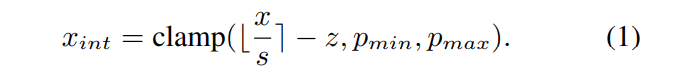
    clamp 함수는 rounded value $\lfloor{\frac{x}{s}-z}\rceil$를
    $[p_{min}, p_{max}]$ 범위로 자른다.

  • layer안의 weight tensor와 activation tensor를 위한 quantization parameters를 설정하기 위해서,
    가장 간단하고 효율적인 방법은 quantization 이전과 이후의
    tensors의 MSE를 최소화하는 quantization parameter를 찾는 것이다.
    $\\$
    다른 방법으로, L1 distance, cosine distance, KL divergence도
    quantization 전후의 tensors 간의 distance를 측정하는데 사용될 수 있다.

• 신경망의 activations를 계산하기 위해선,
  적은 수의 calibration samples가 PTQ의 input으로 사용돼야 한다.
  선택된 quantization parameters는 calibration samples 선택에 의존적이다.

• ZSQ(Zero-shot quantization)는 PTQ의 특수한 케이스다.
  ZSQ는 신경망에 기록된 정보(예를 들면, batch normalization layer의 mean과 var)에 따라
  calibration dataset을 생성한다.
  $\\$
  real samples의 distribution과 유사하도록 activations의 distribution을 만들기 위해서,
  gradient descent를 통해 input sample을 생성한다.
  $\\$
  diffusion 모델에서 noise로부터 image를 생성하는 과정은
  오직 network inference만 사용하기 때문에,
  이전의 ZSQ methods와는 꽤 다르다.

PTQ on Diffusion Models

Preliminaries

PTQ

• well-trained network의 각 layer의 weight tensor와 activation tensor를 위한 quantization parameters를 선택한다.

• 본 연구에서는 tensor를 quantized tensor로 변환하기 위한
  quantization parameter로
  scaling factor $s$와 zero point $z$를 사용했다.

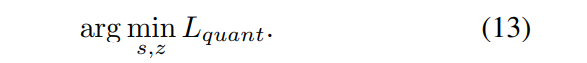
  • quantization으로 인한 error를 최소화하는 것은
    quantization parameters를 선택하기 위해 가장 널리 쓰이는 방법 중 하나이다.
    $\\$
    quantization error는 아래와 같이 수식화된다.
    
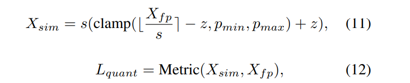
    $X_{sim}:$ deqauntized tensor
    Metric: fp tensor $X_{fp}$와 $X_{sim}$의 distance를 측정하기 위한 metric 함수
    (MSE, cosine distance, L1 distance, KL divergence는 널리 쓰이는 metric functions이다.)

  • quantization 과정은 아래 같이 수식화 될 수 있다.
    
    quantization error를 최소화하기 위해 weight를 direct하게 quantize할 수 있지만,
    우리는 input 없이는 바로 activation tensor를 얻고 quantize 할 수는 없다.
    

  • 따라서 fp activation tensor를 모으기 위해서,
    unlabeled input samples(calibration dataset)이 input으로 사용된다.
    calibration dataset의 크기는 (e.g. 128 randomly selected images) training dataset에 비해 무척 작다.

• 보통, PTQ는 신경망을 세 단계로 quantize한다.

  • 1) 신경망에서 어떤 operation이 quantized되어야 하는지 고르고,
    다른 opeartion들은 fp로 냅둔다.
    $\\$
    예를 들어,
    softmax와 GeLU와 같은 특별한 함수들은 fp로 냅둔다.
    이 operation들을 quantize하면 심각하게 quantization error를 증가시킬 수 있고, 연산이 그렇게 많이 요구되지 않기 때문이다.

  • 2) calibration sample들을 모은다.
    calibration samples에 quantization parameters가 overfitting되지 않도록 하려면,
    calibration samples의 distribution은 real data의 distribution과 가능한한 가까워야 한다.

  • 3) weight tensors와 activation tensors를 위한
    quantization paramers를 선택하기 위해 적절한 방법을 사용한다.

Exploration on Operation Selection

• diffusion model에서 어떤 operations가 quantized되어야 하는지 image generation procss를 분석했다.

• diffusion model은 iterative하게 $x_t$로부터 $x_{t-1}$를 생성한다.
  각 timestep에서, 신경망의 inputs는 $x_t$, $t$이고
  outpus는 mean $\mu$와 variance $\Sigma$이다.
  $\\$
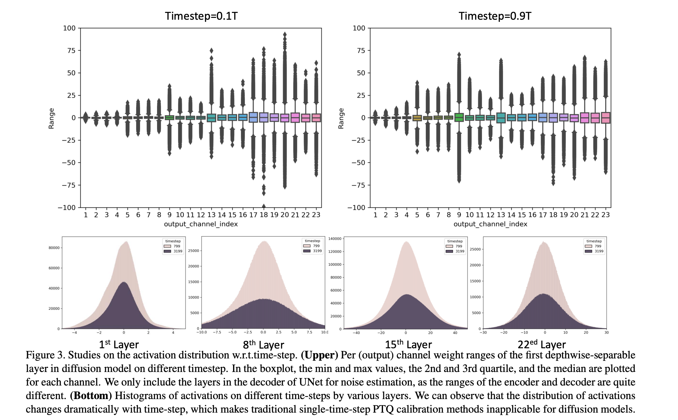
  $x_{t-1}$은 아래 수식에서 정의된 distribution으로부터 sampling 된다.
  
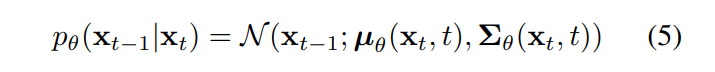
  Figure. 2와 같이, diffusion model의 신경망은 UNet 형태의 CNN 구조를 갖는다.
  
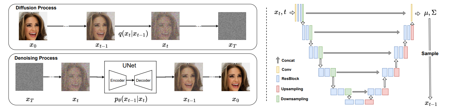
  이전 PTQ 연구들과 같이, computation-intesive conovlution layers와 fully-connected layers는 quantized되어야 한다.
  batch normalization은 convolution layer안에 포함될 수 으며,
  SiLU와 softmax같은 특수한 함수는 full-precision으로 유지된다.

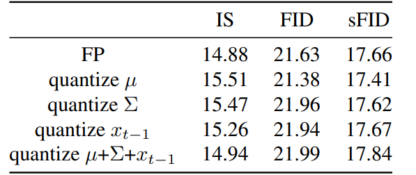
• diffusion model에 두 가지 질문이 더 있다.

1. 신경망의 output인 $\mu$와 $\Sigma$가 quantized될 수 있을까?
2. sampled image $x_{t-1}$이 quantized될 수 있을까?
   $\\$
   이에 대해 답하기 위해서,
   우리는 오직 $\mu$, $\Sigma$ 또는 $x_{t-1}$을 생성하는 operation을 quantize한다.
   $\\$
   Table 1과 같이, $\mu$, $\Sigma$ 또는 $x_{t-1}$들은 quantization에 민감하지 않음을 관찰했고,
   quantized될 수 있음을 알 수 있었다.
   

Exploration on Calibration Dataset

• 두 번째 단계는 diffusion model을 quantize하기 위한 calibration sample들을 모으는 것이다.

  calibration samples는 training dataset으로부터 얻어질 수 있으며, 다른 networks를 quantize하는데 사용된다.

  하지만, diffuion model의 training dataset은 $\bold{x_0}$로, network's의 input이 아니다.
  실제 input은 genrated smaples $\bold{x_t}$이다.

  또한, 우리는 diffusion process의 generated samples를 사용해야 할까?
  또는 denoising process의 generated samples를 사용해야 할까?

  어떤 time-step $t$에서, generated samples를 뽑아야 할까?

  이 section은 어떻게 좋은 calibration dataset을 만들 수 있는지 살펴본다.
  

• 여러 PTQ baseline들을 조사하여 네 가지 유의미한 관찰(아래 Analysis on PTQ calibrations and DMs)을 얻어서, 본 연구의 설계에 참고했다(아래 Noramlly Distributed Time-step Calibration).

  PTQ4DM calibration을 통해, 8-bit PTQ diffusion model은 full-precision 모델과 동일한 성능을 가짐을 실험을 통해 알 수 있었다.
  (8-bit DM 23.9 FID, 15.8 IS
  32-bit DM 21.6 FID, 14.9 IS)

Analysis on PTQ Calibration and DMs

• 우리는 뽑은 calibration sample들의 distribution이 real data의 distribution과 가능한한 가깝길 원한다.
  calibration set이 quantization error를 줄이도록 quantization을 supervise할 수 있기 때문이다.

  이전의 연구들은 single-time-step 시나리오에서 구현되었기 때문에,real training dataset으로부터 networks를 quantizing하기 위한 sample들을 직접 추출할 수 있었다.

  calibration dataset은 굉장히 작은 규모이기 때문에, colletcion은 굉장히 sensitive하다.
  만약 뽑은 calibration dataset의 분포가 real dataset을 잘 표현(반영)하지 못한다면, calibration task에 overfitting을 초래할 수 있다.
  

• DM을 위한 PTQ를 calibration할 때는 더 많은 challenge가 존재한다.
  quantize될 networks의 input들이 generated samples $\bold{x_t} (t=0, 1, ..., T)$이다.

  DM을 quantize하기 위해선 calibration dataset collection method를 특정한 multi-time-step 시나리오에서 고안해야 한다.

  이 연구에선 PTQ calibraion과 DMs를 모두 조사한 후, 다음과 같은 관찰을 얻을 수 있었다.
  

Observation 0: Distributions of activation changes along with time-step chaning.

• diffusion model들의 output distribution 변화를 이해하기 위해, time-step에 따른 activation distribution을 조사했다.

  time-step에 달라짐에 따라 output distribution이 어떻게 변화하는지, 예를 들어
  $t_1 = 0.1T$와 $t_2 = 0.9T$가 주어졌을 때,
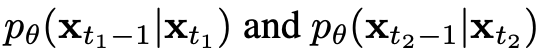  의 output activation distribution을 분석하고자 했다.

  이론적으로, time-step에 따라 distribution이 변화한다면,
  이전의 PTQ calibration methods들은 temporally-invariant calibration으로 제안되었기 때문에 적용하기에는 어려움이 있다.

  먼저 noise estimatio network의 overall activation distribution을 boxplot을 통해 분석했다.
  그 후 histogram을 통해 layer-wise distributions를 면밀히 살펴봤다.
  그 결과는 다음 Fig 3과 같다.
  각기 다른 time-steps에서 대응되는 activation distributions는 큰 차이를 갖고있음을 알 수 있었고,
  이전의 PTQ calibration methods들을 DM과 같은 multi-time-step models에 적용이 어려움을 알 수 있었다.
  

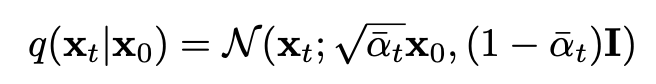
Observation 1: Generated samples in the denoising preocss are more constructicve for calibration

• 보편적으로, diffusion에서 PTQ calibration을 위한 sample들을 생성하는 데는 두 방향이 있다.
  1) raw images as input for diffusion process
  2) noise as input for denoising process

  이전의 PTQ methods들은 raw image들을 사용했는데,
  raw images는 training set의 distribution을 대표할 수 있는 GT 역할을 할 수 있기 때문이다.

  본 연구는 각각 raw images for diffusion process와
  Gaussian noise for denoising process로 이루어진 두 가지 calibration sets로 quantized model들을 calibrate하는 비교 실험을 진행했다.

  또 다른 유사한 baseline은 diffusion process의 training samples를 calibration data로 사용한다.
  구체적으로 말하면, 우리는 각 image $\bold{x_0}$에 대해 timestep $t$를 랜덤하게 생성하고,
  아래 수식을 사용해 $\bold{x_t}$를 생성한다.
  
  다르게 말하면, Image + Gaussian 에서 calibration samples를 추출하는 것이다.
  이를 training-mimic baseline으로 명명했다.

  실험 결과는 아래 Tab. 2.에 나와있다.
  이 실험을 통해 diffusion process의 input noise가 quantized DMs를 calibration하는데 더 효율적임을 알 수 있었다.
  
  

Observation 2: Sample $\bold{x_t}$ close to real image is more benefical for calibration.

• 위 관찰을 바탕으로, 각 time-step $t$의 samples로 calibrated되는 quantized diffusion model인
  DM을 위한 PTQ calibration baseline을 만들었다.
  이때, [Loss aware post-training quantization] 논문을 기반으로 했다.
  이 straight-forward한 접근을 naive PTQ-for-DM baseline으로 명명했다.

  구체적으로, Gaussian noise $\bold{x_t} \sim N(0, \bold{I})$가 주어질 때,
  calibration set을 $\bold{x_t}$로
  생성하기 위해, 아래 Eq. 5의 full-precision noise estimation network $p_{\theta}(\bold{x_{t-1}|x_t})$를 사용하는 diffusion model을 사용했다.
  

  그 후, calibration set을 사용해서 우리의 quantized noise estimation network, $p_{\theta'}(\bold{x_{t-1}}|\bold{x_t})$를 calibrate하기 위해 사용했다.
  (여기서 ${\theta'}$은 quantized paramters를 뜻한다.)

• 이 calibration baseline과 함께 각기 다른 time-steps에서 일련의 실험을 진행했다.
  $i.e., t=0.0T, 0.2T, ..., 1.0T$
  where $T$: total denoising time steps.

  이 실험의 결과는 아래 Fig.4와 같다.
  naive baseline으로 calibrated된 8-bit 모델은 만족할만한 image를 정성적으로나 정량적으로 생성하지 못함을 확인할 수 있다.
  

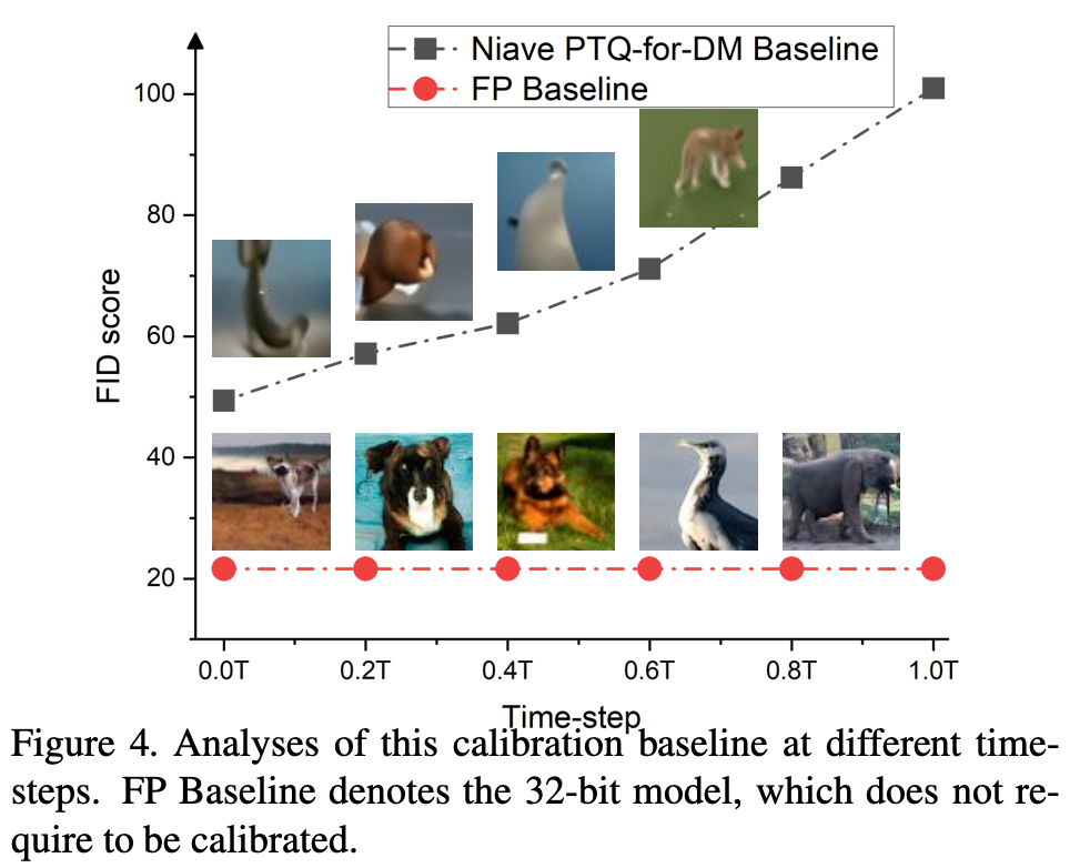
  다행히도, 이 실험을 진행하면서 PTQ calibration이 time-step $t$가 real image $\bold{x_0}$에 다가가면서 더 도움이 된다는 점을 알 수 있었다.

  이 현상에 대한 직관적인 설명을 해보자면,
  denoising process에서 $t$가 줄어들면서, network $p_{\theta}(\bold{x_{t-1}}|\bold{x_t})$의 output의 distribution은 real image의 distribution과 유사해지기 때문이다.

Observation 3: Instead of a set of samples generated at the same time-step, calibration samples should be generated with varying time-steps.

• 대부분의 methods들은 single-time-step 시나리오를 위해 제안되었지만,
  본 연구의 calibration dataset은 multi-time-step 시나리오를 위해 뽑았다.

  본 연구에서는 diffusion model의 calibration dataset은 다양한 time-stpe의 sample stem을 포함해야 한다고 가정했다.
  time-step에 따른 sample의 차이를 반영해야 된다고 생각했기 때문이다.
  가장 직관적으로 이 가정을 실험해볼 수 있는 방법은 time-steps의 범위에서 uniform하게 $t$를 sampling하는 것이다.
  

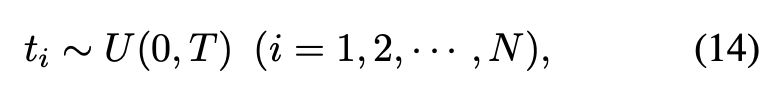
여기서 $U(0,T)$: uniform distribution between 0 and T,
$N$: size of calibration set,
$T$: # of time-steps in denoising process

주어진 Gaussian noise $\bold{x_t} \sim N(0, \bold{I})$와 $t_i$에 대해서,
full-precision noise estimation network $p_{\theta}(\bold{x_{t-1} | x_t})$로 diffusion model을 사용하여,
$\bold{x_{t_i}}$를 생성한다.

최종적으로, calibration set $C = {\bold\{x_{t_i}}\}^N_{i=1}$을 얻게 된다.
따라서 위 calibration sample은 넓은 범위의 time steps를 커버할 수 있다.

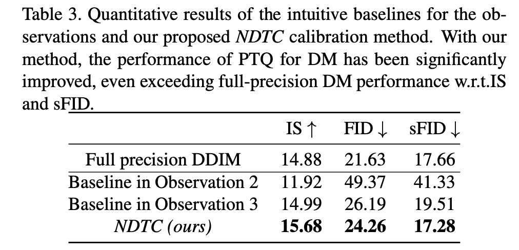
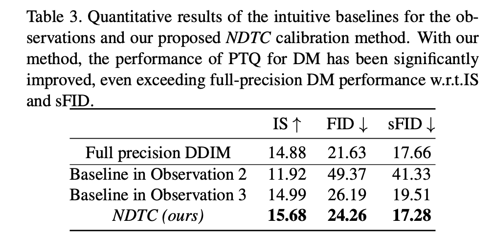
이 collection method의 효율성을 테스트한 결과는 Tab. 3과 같다.
결과적으로 time-step discrepancy를 반영하는 calibration sample들을 validate하는 결과를 얻었다.

Normally Distributed Time-step Calibration

• 위에서 증명한 calibration baseline과 observation을 바탕으로, calibration sample이 다음을 만족하길 원한다.
  1) full-precision diffusion model로 denoising process에 의행 생성되는 calibration samples
  2) $\bold{x_0}$에 상대적으로 가깝고,
  $\bold{x_t}$로부터 멀리 떨어진 calibration samples.
  3) 다양한 time-steps를 커버한 calibration sampels.

  하지만 위의 2), 3) 조건은 trade-off 관계로, 동시에 수행될 수 없다.

  모든 조건을 고려하여, DM-specifig calibration set collection method를 제안하는데,
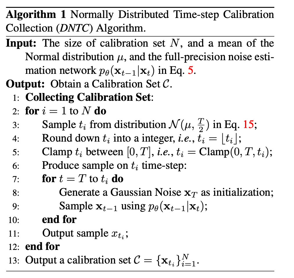
  그 이름은 Normally Distributed Time-step Calibration(NDTC)이다.

  이 method는 calibration set ${x_{t_i}}$가 denoising pocess에 의해 생성되고(조건 1),
  이때 time-step $t_i$는 skew Normal distribution으로부터 샘플링된다.
  (조건 2와 3의 균형을 맞추기 위해서)

  구체적으로, time-step 범위에서 skew normal distribution을 따르는 sampled ${t_i}$를 생성한다.
  

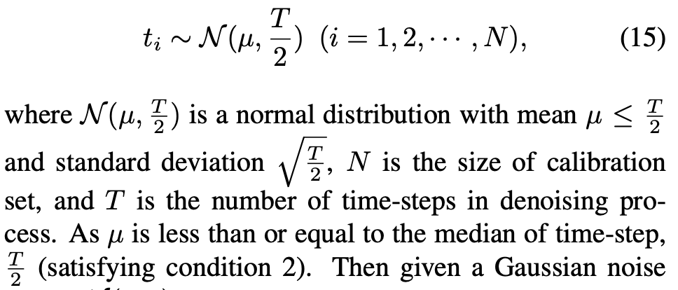
이후, 주어진 Gaussian noise $\bold{x_T} \sim N(0, \bold{I})$와 $t_i$로,
full-precision noise estimation network$p_{\theta}(\bold{x_{t-1}|x_t})$와 함께 diffusion model을 사용하여, $x_{t_i}$를 생성한다.

최종적으로, 우리는 calibration set $C = \{\bold{x_{t_i}}\}^N_{i=1}$을 얻게된다.
자세한 collection 알고리즘은 아래와 같다.

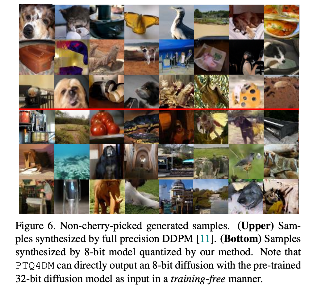
NDTC의 효율성은 PTQ baseline과 full-precision DM 간의 비교를 통해 평가했으며,
결과는 Tab.3, Fig.6와 같다.

Exploration on Parameter Calibration

• calibration sample들이 collected되면,
  세 번째 step은 diffusion mdoel의 tensor들을 위한 quantization parameter를 선택하는 것이다.

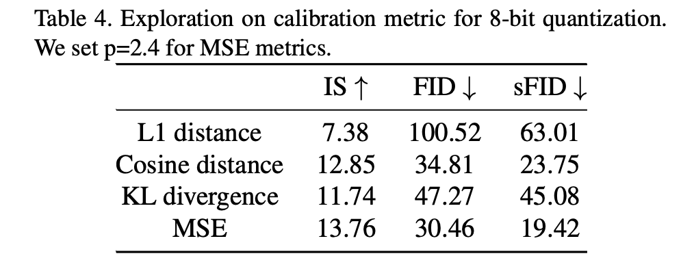
• Table 4에서 볼 수 있듯,
  MSE가 L1 distance, cosine distance, KL divergence보다 보다 더 나은 것을 확인했고
  MSE를 diffusion model을 quantize하는 metric으로 사용했다.