Abstract

noise estimation model의 low inference, high memory consumption, and computation intensity가 diffusion model의 효율적인 adoption을 방해하는 요소이다.

PTQ가 다른 task들에 대해선 go-to compression 방법으로 자리 잡았지만, diffusion model은 아직 out-of-the box이다.

generation procss를 accelerate하기 위해 noise estimation netowrk를 compression하는 PTQ 방법론을 제시한다. 이는, diffusion 모델의 unique한 multi-timestep pipeline과 모델 architecture를 specifiaclly tailor한다.

diffusion model의 key difficulty는 아래와 같다.
1) noise estimation network의 multiple한 time step에 걸쳐 변환하는 output distribution
2) noise estimation network의 shortcut layer들의 bimodal activation dsitribution

우리는 이 challenge들을 다루고자,
timestep-aware calibration과 split short-cut quantization을 제시한다.

실험 결과 우리 방법론은 training-free manner로
full-precision의 unconditional diffusion model을
comparable performance를 유지하며 4-bit로 quantize 함을 보였다.
또한, 처음으로 4-bit wegiths로 stable diffusion을 구동해
high generation quality를 생성하도록 text-guided image generation에 적용될 수 있다.

Introduction

[diffusion model에 Quantization이 필요한 이유]

복잡한 신경망을 이용한 50번부터 1000번 time step의 반복적인 noise estimation network로 인해 generation process가 slow down된다.

이전의 SoTA 접근들(예를 들면 GAN)은 multiple한 image를 1초 이내로 generate할 수 있는 반면,
diffusion은 single image를 sampling하기 위해 보통 몇 초가 걸린다.
결과적으로, image generation process를 speed up하는 것은 중요한 과제다.

이전의 연구들은 더 짧고 효율적인 sampling 경로를 찾는 방식으로 denoising process의 step 횟수를 줄이는 방식으로 이 문제를 해결하려 했다.
하지만, 이 연구들이 크게 간과한 점이 있다.
각 iteration 자체에서 noise estimation model 그 자체가 compute-, memory-intensive하다는 점이다.
이는 diffusion model의 inference를 slow down할 뿐 아니라, high memory footprints 관점에서도 crucial한 challenge이다.

[Q-Diffusion의 접근 방식]

PTQ4DM은 diffusion model을 8-bit로 compression 했지만,
smaller dataset과 lower resolution에 집중했다.

Chanllenges
우리는 PTQ4DM과 동시에 발전하면서,
1) 각 time step마다 noise estimation network의 output distribution이 largely different 함을 발견했다.
$\rightarrow$ 따라서, 이전의 PTQ 방법론을 적용하는 것은 성능 하락 요인이 된다.

2) noise estimation network의 iterative inference는 quantization error의 accumulation을 초래한다.
$\rightarrow$ noise estimation network를 위한 calibration objectives와 quantization scheme 설계가 요구된다.

Approach
이러한 Challenge들을 다루기 위해서,
data-free manner로 noise setimation을 compression하는 Q-Diffuion을 제시한다.

1) pre-trained diffisoin model로부터의 time step-aware calibration data sampling 메커니즘을 제안한다.
이는 모든 time step들의 activation distribution을 represent한다.

2) 흔히 사용되는 noise estimation moedl architecture의 quantization error을 줄이기 위해, calibration objective와 weight and activtaion quantizer를 tailor 한다.

성과
pixel-space와 latent-space unconditonal diffusion model에 대해 W4A8 PTQ를 가능케 한다.
(full precision model과 비교해서 FID increment가 0.39-2.34 정도만 되면서.)

Related Works

Diffusion Models
UNet이 diffusion model에서 noise estimation model로 많이 쓰임.
최근에는 Transformer를 사용하는 연구들이 제시 되기도 함.
이 연구는 가장 흔히 사용되는 UNet으로 된 noise estimation network를 acceleration하고자 함.

Accelerated Diffusion Process

• non-Markovian process로 generalize하여 더 적은 step으로 diffusion process를 simulating하는 연구

• variance schedule을 조절하거나, high-order solver를 사용해 diffusion generation을 approximate하는 연구

• feature maps을 caching하고 reusing하는 기술 연구

• diffusion model을 distill해서 더 적은 time step으로 만드는 연구
  주목할만한 성취를 거뒀지만, extremely expensive retraining 과정이 필요함.

우리 모델은 training-free PTQ process로
각 step의 noise estimation model inference를 accelerating하는데 foces함.

Post-training Quantization

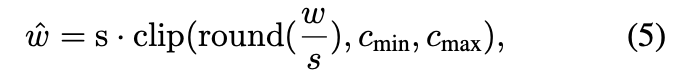
PTQ는 $w$를 discrete한 set of values로 rounding하여 신경망을 compression함.
quantization과 de-quantization은 다음과 같이 공식화됨.

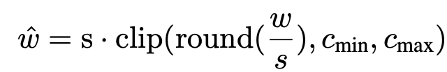
$s$: quantization scale parameters
$c_{min}, c_{max}$: clipping 함수 $clip(\cdot)$의 lower, upper bounds.
이 parameter들은 PTQ process 안에서 estimated된 weight과 activation distribution을 사용해서 calibrated될 수 있음.
$round(\cdot)$은 rounding-to-nearest 또는 adptive rounding 연산임.

classification과 detection task의 이전 PTQ 연구들은 calibration objective와 calibration data를 얻는 것에 focus함.
예를 들어, EasyQuant는 training data를 기반으로 적절한 $c_{min}, c_{max}$를 결정한다.
BRECQ는 Fisher information을 objective에 도입했다.
ZeroQ는 distllation 기술을 활용해서 PTQ를 위한 proxy input image를 생성한다.
SQuant는 Hessian sectrum을 통해 결정된 sensitivity를 토대로 한 objectoive에 random sample을 사용한다.

diffusion model quantization의 경우, training dataset이 필요하지가 않다. 왜냐하면 random inputs를 사용한 full-precision 모델에서 sampling 하여 calibration data를 만들 수 있기 때문이다.
하지만, noise estimation 모델의 multi-time step inference는 activation distribution을 modeling하는데 새로운 challenge를 가져온다.

이 연구와 parallel한 PTQ4DM은 Normally Distributed Time-step Calibration 방법을 도입해서, specific한 distribution을 사용해 모든 time step에 걸쳐 calibration data를 생성한다.
그럼에도 불구하고, 이러한 접근은 lower resolutions, 8-bit precision, float-point attention activation-to-activation matuls로 제한된다.
그리고 다른 calibration scheme들과의 ablation study도 제한적이다.
이 방법을 더 낮은 precision에 적용했을 때, 결과는 더욱 worsek하다.

우리 연구는 calibration dataset creation의 implication을 holistic한 방법으로 파고든다.
diffusion model을 위한 효율적인 calibration objective를 설계하는 것이다.
우리는 fully하게 act-to-act matmuls를 quantize한다.
그리고 이를 512 x 512 resolution 까지되는 large-scale dataset에 pixe-space와 latent-space diffusion model 모두 포함해 실험을하여 증명했다.

Method

multi-step inference 과정과 noise estimation network로 사용되는 UNet 구조에 대해
Section 3.1과 Section 3.2에서 각각 분석하고
full Q-Diffusion PTQ pipeline을 Section 3.3에서 분석한다.

3.1 Multi-step Denoising에서의 Chanllenge들

우리는 multi-step inference process를 사용하는 quantizing model들의 두 가지 주요 challenge를 소개한다.

Challenge 1: Quantization error가 time step에 걸쳐 누적된다

신경망에 quantization을 수행하는 것은 well-trained model의 weight과 activation에 noise를 초래해, 각 layerdml ouput에 quantization error를 초래한다.
이전 연구에서 quantization error는 layer를 거치며 누적되기 쉽기 때문에, deep한 신경망을 quantization 하는 것이 더 어려움을 밝혔다. [6]
diffusion model의 경우, 어떤 time step $t$에서, denoising model의 input $\bold{x}_t$는 $\bold{x}_{t+1}$로부터 얻어진다.
이 과정은 연산에 포함되는 layer들의 갯수를 denoising steps에 비례해 multiply한다. 긜고 이는 denoising 과정의 나중 step으로 갈수록 quantization error를 누적한다.

우리는 CIFAR-10 데이터셋에 대해 64 batch size로 DDIM의 denoising process를 실행했다.
그리고 각 time step에서 full-precision 모델과 INT8, INT5, INT4로 quantized된 모델들의 MSE 차이를 비교했다.

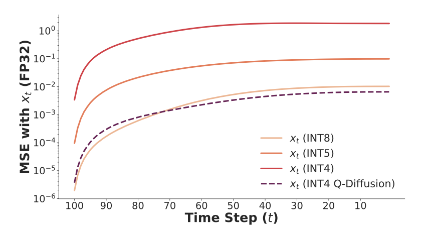
Figure 3에서 볼 수 있듯, 모델이 4-bit로 quantized될 때 dramatic한 quantization error의 증가를 볼 수 있다. 그리고, error가 iterative denoising을 거치면서 빠르게 누적되고 있음을 볼 수 있다.
이는 모델을 low precision으로 quantizing한 이후에 성능을 유지하는데 어려움을 초래한다.
따라서 모든 time step에서 quantization error를 가능한 줄이는 것이 필요하다.

Challenge 2: Activation distribution이 time step에 걸쳐 vary하다

각 time step에서 quantization error를 줄이기 위해, 이전의 PTQ 연구들에서는 quantized된 모델을 a small set of calibration data로 clipping range와 scaling factor를 calibrate한다.
calibration data는 적절한 calibration을 위해 모델의 activation distribution이 correctly하게 estimated될 수 있도록, 실제 input distribution과 닮도록 sampling되어야 한다.

Diffusion 모델이 모든 time step들에서 input을 구하기 위해 동일한 noise estimation netowrk를 사용한다는 점에서, 각기 다른 time step에서 data를 sampling하는 방법을 결정하는 것은 중대한 challenge가 된다.

우리는 각기 다른 time step에 걸쳐 UNet 모델의 activation distribution을 분석하는 것으로 시작했다.
DDIM을 이용해서 100 denoisiing step으로 위에서 진행한 동일한 CIFAR-10 실험을 진행했고,
모든 time step 중에서 1000개의 random sample들의 activation range를 구했다.
아래 Figure 5 에서 볼 수 있듯, activation distribution은 gradually하게 변했다.
가까운 주변의 time step에서는 유사하고, 멀리 떨어진 time stepd은 차이가 구별됨을 알 수 있다.

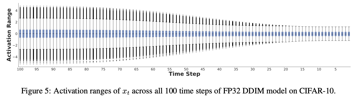
output activation distribution이 time step을 거치며 vary하다는 사실은 quantization에 challenge다.
denoising 과정에서의 noise estimation model에 의한 모든 time step full range의 activation을 반영하지 않는, 오직 적은 몇 개의 time step을 사용해서 noise estimation model을 calibration하는 것은
특정 time step에 의해 묘사된 activation distribution에 overfitting을 유발할 수 있고, 다른 time step들에 잘 generalize되지 않을 것이다.

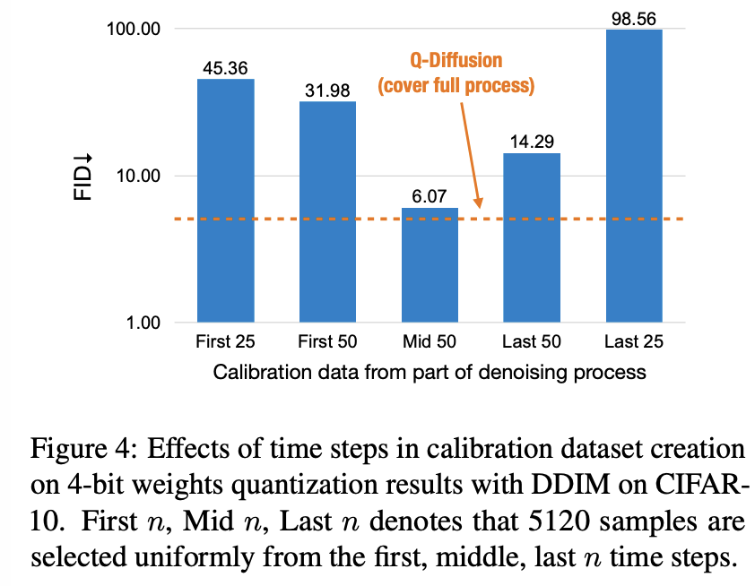
예를 들어, denoising process에서 각기 다르게 sampling된 data로 진행한 CIFAR-10 데이터셋을 사용한 Quantized DDIM을 calibrate를 시도했다.
Figure 4에서 볼 수 있듯, 우리는 denoising process의 특정 단계에 속하는 time step들로부터 5120개의 sample들을 단순히 sampling 했다. 그리고 이는, 4-bot weoghts quantization 하에서 significant한 성능 하락을 유발했다.
주목할 점은 '중간의 50개 time step으로부터 샘플링한 경우'가 처음 또는 마지막 n 개의 time step에서 sample을 추출한 경우보다 더 적은 성능 하락을 보였다.
이는 Figure 5에서 본 gradual한 denoising process를 반영하는 결과이다.
activations distribution이 time step에 따라 gradually하게 변화하므로, 중간 부분이 어느 정도 full range을 capturing하는 것이다. (거리가 먼 endpoints는 가장 차이가 큰 반면)
qunatized diffusion 모델의 성능을 회복하기 위해선, 우리는 각기 다른 time step 들의 output distribution을 comprehensive하게 고려해서 calibration data를 선택해야 한다.

3.2 Noise Estimation Model Quantization의 Challenges

대부분의 diffusion 모델들 (Imagen, Stable Diffusion, VDMs)은 latent feature들을 downsample하고 upsample하는 denoising backbone으로 UNet을 사용한다.
최근 연구들에서는 transformer 구조도 noise estimation backbone으로 사용할 수 있음을 제시하고 있지만, 현재까지 UNet은 표준이 되는 구조이다.
UNet은 concatenated된 deep feature와 shallow feature들을 merge하고, subsequent layer들로 transmit하기 위해서 shortcut layer들을 사용한다.

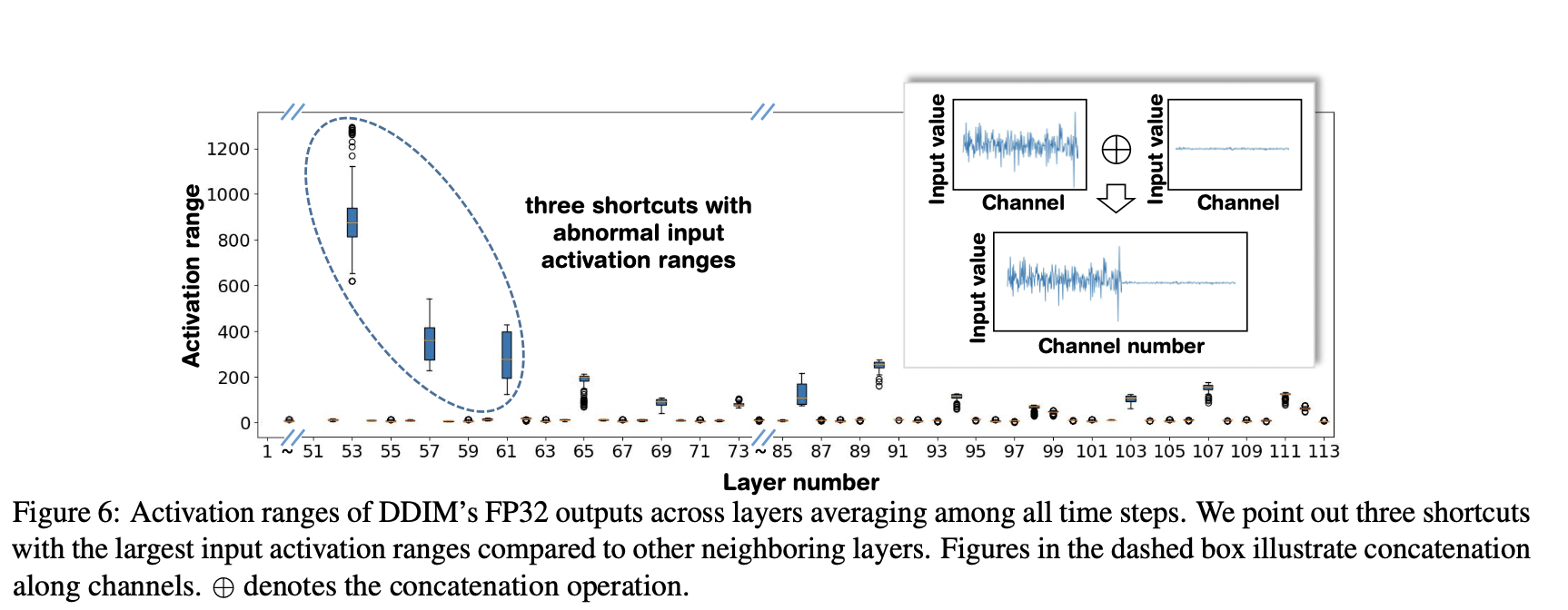
Figure 6에 제시된 우리의 분석을 통해 우리는 shortcut layer 안의 input activation들이 다른 이웃한 layer들과 비교했을 때, abnormal한 value ranges를 보임을 관찰했다.
DDIM의 shortcut layer들의 input activation은 다른 이웃한 layer들보다 200배 더 larger하다.

이 원인을 분석하기 위해서, 우리는 DDIM shortcut layer의 weight과 activation tensor를 visualize했다.
Figure 6의 dashed box에서 알 수 있듯, deep feature channels ($X_1$)와 shallow feature channels ($X_2$)로부터의 activation range가 함께 concatenated되어 significant하게 vary한다.
이는 대응되는 channels의 bimodal weight distribution을 초래한다. (Figure 7에서 볼 수 있듯)

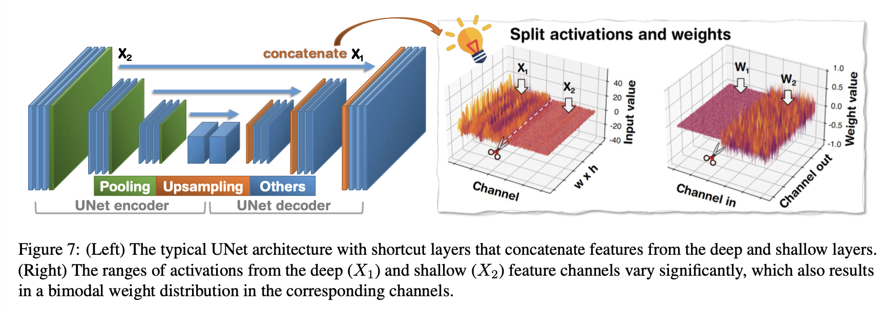
Naive하게 전체 weight과 activation distribution을 동일한 quantizer로 quantizing하는 것은 large quantization error를 초래할 것이다.

3.3 PTQ of Diffusion model

우리는 두 가지 기술을 제시한다.
1) time step-aware calibration data sampling
2) shortcut-splitting quantzation

3.3.1 Time step-aware calibration
연속적인 time setp들의 output distribution이 종종 거의 유사하기 때문에,
우리는 모든 time step들의 fixed interval에서 intermediate inputs을 uniformly하게 random sampling해서 작은 calibration set을 만드는 것을 제안한다.
이는 calibration set의 크기와 calibration set의 모든 tim setps에 걸친 distribution을 표현하는 능력 간의 효율적인 균형을 맞춘다.
경험적으로, 우리는 sampled된 calibration data가 calibration 이후에 대부분의 INT4 quantized model 성능을 recover 할 수 있음을 발견했다.
따라서 이는 quantizatoin error correction을 위한 calibration data collection을 위한 효율적인 sampling scheme이라고 할 수 있다.

quantized model을 calibrate하기 위해, 우리는 model을 여러 개의 reconstribution blocks로 divide하고, iterative하게 outputs를 reconstruct 했으며, adptive rounding과 함께 각 block weight quantizer clipping range와 scaling factor를 tuning해서
quantized output과 full precision ourtput 사이의 MSE를 최소화하도록 했다.

우리는 Residual Bottleneck Block 또는 Transformer Block과 같이
diffusion model 안의 residual connections Unet을 block으로 포함하는 core component를 정의 했다.
모델에서 이 조건을 만족하지 않는 다른 부분들은 per-layer 방식으로 calibrate됐다.
이 기술은 fully하게 layer-by-layer calibration을 하는 방식보다 성능을 향상함을 보였다. 왜냐하면 이 방식은 layer 간의 depedency들과 generalization을 addrss하기 때문이다.

acitvation quantization에 관해서는, activations가 inference 도중 constantly하게 변화하기 때문에, adaptive rounding을 하는 것이 feasible하다.
따라서, 우리는 Learned Step Size Quantization을 따라 activation quantizer의 step size를 adjust한다.
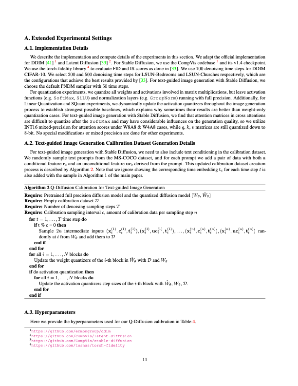
overall한 calibration workflow는 Alg.2.에 제시돼있다.

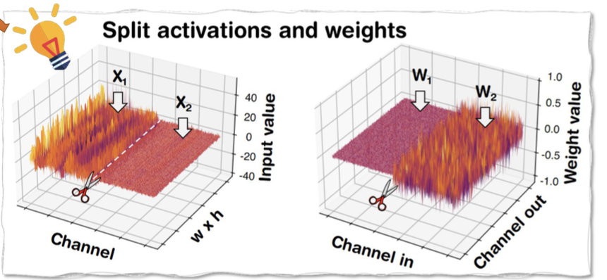
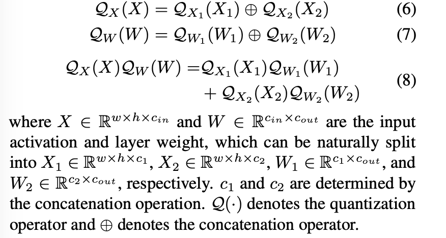
3.3.2 Shortcut-splitting quantization

shortcut layer들에서의 abnormal한 activation과 weight distribution을 address하기 위해,
우리는 concatenation 이전에 quantization을 수행하는 "split" quantization technique을 제안한다.
이는 거의 무시할 수 있는 만큼의 추가적인 메모리 또는 computational resource들이 요구된다.
이 전략은 shortcut layer들에서의 activation과 weight quantization 모두에 적용될 수 있고, 수학적으로는 다음과 같이 표현된다.

Experimetns

4.1 Experiments Setup

제안한 Q-Diffusion 프레임워크를 unconditional image generation을 위한
pixel-space diffusion 모델인 DDPM과
latent-space diffusion 모델인 Latent Diffusion 모델에 적용해 ㅠ평가했다.

또한, Stable Diffusion에 적용한 Q-Diffusion으로 생성된 image를 시각화했다.

지금까지 diffusion model의 quantizatoin 연구가 없었기 때문에,
우리는 basic한 channel-wise Linear Quantization(i.e. Equation5)을 baseline으로 보고했다.

우리는 SoTA data-free PTQ 방법인 SQuant를 re-implemetn하고
비교를 위해 결과를 포함시켰다.

나아가, Q-Diffusion 방식을 Stable Diffusion으로 text-guided image synthesis에 적용했다.

실험결과 모든 task에서 full-precision 시나리오에 가까운 generation quality를 달성했고,
심지어 weights에 대해서 INT4 이하의 quantization에서도 이를 달성했다.

4.2 Unconditional Generation

Dataset

• 32 x 32 CIFAR-10
• 256 x 256 LSUN Bedrooms
• 256 x 256 LSUN Church-Outdoor

CIFAR-10 실험에 pretraiend DDIM sampler와 100 denoising time step을 사용했다.
그리고 Latent Diffusion(LDM)을 higher resolution LSUN 실험을 위해 사용했다.

CIFAR-10에 대한 성능을 FID(Frechet Inception Distance)로 평가하고,
추가적으로 Inception Score(IS)를 평가했다.
왜냐하면 IS는 ImageNet의 domain과 categories로부터 매우 차이를 갖는 dataset에 대해선 정확한 reference가 아니기 때문이다.
결과는 Tab 1-3과 Figure 8과 같다.
(Bops는 latent diffusion을 위한 decoder dompute cost를 고려하지 않은 하나의 denoising step을 연산한 것이다.)

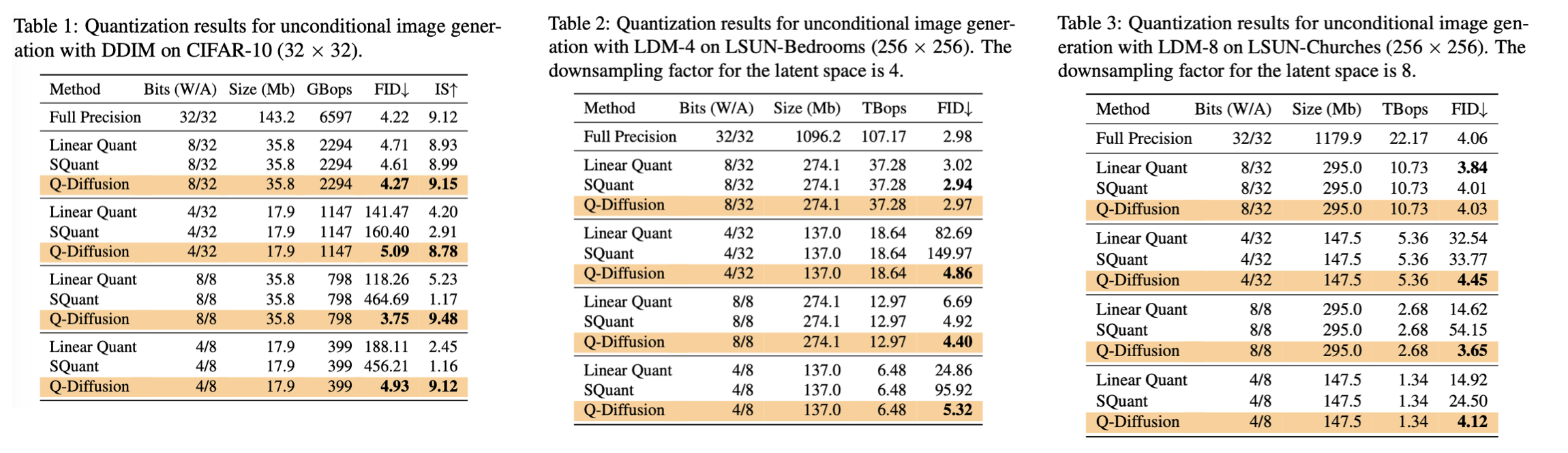
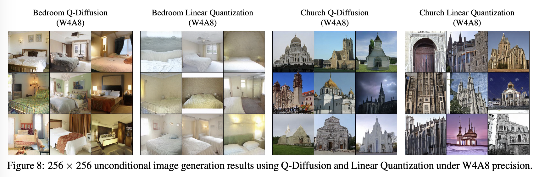
실험은 Q-Diffusion이 significant하게 image generation quality를 preserve함을 보였고,
bit 수가 낮을 때, test한 diffusion 모든 resolution과 type에 대해 Linear Quantization을 large margin으로 outperform함을 보였다.

Linear Quantization과 Q-Diffusion 모두 FP32와 비교해서
8-bit weight quantization이 거의 performance loss가 없음에도 불구하고,
4-bit 이하의 weight quantization의 경우 Linear Quantization의 generation quality가 급격하게 하락했다.
반면, Q-Diffusion은 여전히 대부분의 perceptual quality를 FID가 최대 2.34 증가하는 정도로 quality를 유지했고 imperceptible distortion을 유지했다.

4.3 Text-guided Image Generation

Q-Diffusion을 512 x 512 LAION-5B subset에 pretrained된 Stable Diffusion에 적용해 text-guided image generation을 평가했다.

textMS-COCO로부터 text prompts를 샘플해서 text condition으로 calibration dataset을 생성했다. (Algorithm 1 이용)

Stable Diffusion에서 guidance strength를 default 7.5로 fix했다.

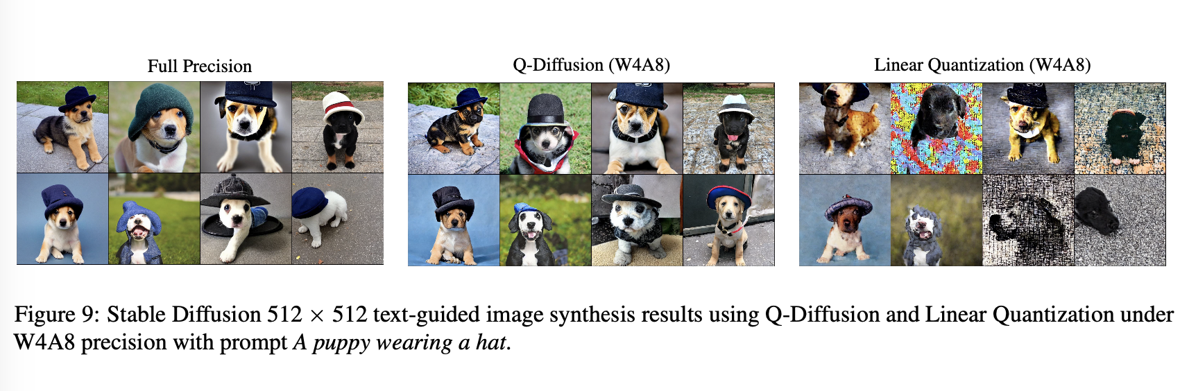
Qulaitative results는 Figure 9와 같다.
Linear Quantization과 비교해서, Q-Diffusion이 더 높은 quality image를 realistic한 detail과 더 나은 semantic information의 demonstration으로 보여줬다.

W4A8 Q-Diffusion 모델의 output은 full precision 모델의 output과 크게 유사했다.

흥미롭게도, 우리는 Q-Diffusion 모델과 FP 모델 사이의 lower-level semantics 에서 some diversity를 발견했다. 예를 들어, horse의 heading이나 hat의 모양같은.
이런 diversity에 quantization이 어떻게 contribute하는지 이해하는 것은 future work로 남긴다.

4.4 Ablation Study

Effects of Sampling Strategy

caliibration을 위한 각기 다른 sampling strategy의 영향을 분석했다.
sampling에 사용된 다양한 time steps 개수와 calibration을 위해 사용된 sample들을 실험했다.

uniform timestep intervals로부터의 calibration sets에 더해서,
우리는 first 50 stes와 last 50 steps에서의 sampling도 시도했다.

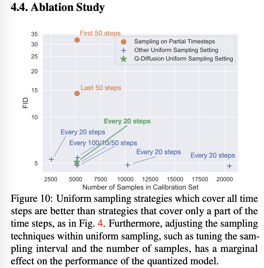
Figure 10처럼, 모든 time step 결과를 span하는 uniform sampling이 오직 부분적인 time stpe로부터 sampling하는 것과 비교해 더 좋은 성능을 보였다.

나아가, calibration sample들을 더 사용하는 것을 포함해 sampling hyperparameter를 조정하는 것은 성능 향상에 큰 영향이 없었다.
따라서, 우리는 calibration을 위해 단순히 총 5120 개의 샘플들에 대해 20 step마다 uniform하게 sampling 했다. 이를 통해 quantization 과정에서 low computational costs로 high-qulaity quantized model 결과를 얻었다.

Effects of Split

이전의 Liniear quantization 접근은 Figure 11과 같이 심각한 성능 하락을 겪었다. (4-bit weight quantization이 DDIM CIFAR-10 generation에서 높은 FID 수치를 보이고 있음)

8-bit activation quantization을 추가적으로 사용하는 것은 더욱 성능을 악화했다.
(FID 수치 더 높아짐)

quatization에서 shorcuts를 splitting하는 것을 통해, generation performance를 significant하게 향상했다.
(FID 4.93 on W4A8 quantization)