https://www.bradyneal.com/causal-inference-course
Introduction to Causal Inference라는 강의를 듣고 정리했습니다.

6. Estimation

6-1. Preliminaries

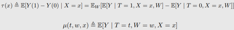
Condiitional average treatment effects(CATEs)

• individualized average treatment effect

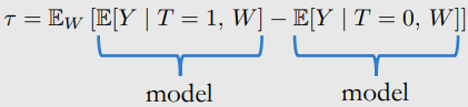
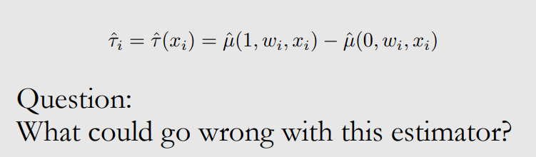
6-2. Conditional Outcome Modeling(COM)

• 아래 conditional expectation을 modeling 해야함.
  
  
• i : data sample
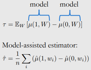
• linear regression으로 modling 함
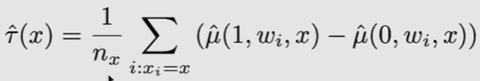
• COM estimation of CATEs
  • CATE Estimand
    
  • CATE COM Estimator
    
  • ITE
    

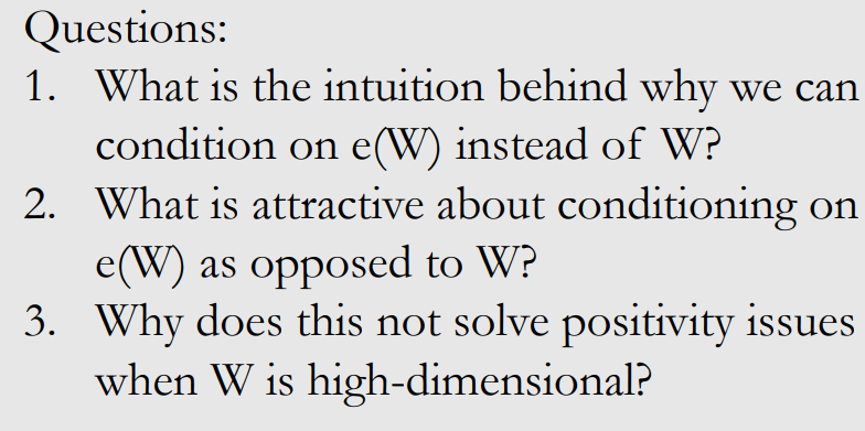
질문이 뭐지?

• 여러가지 이름
  • G-Computation estimators
    • Generalize : time varying treatment의 generalization
    • G-estimation이랑 헷갈림
  • Parametric G-formula
  • Standardization
  • S-learner where 'S' is for 'Single'

고차원에서 COM estimation의 문제

• T는 무시되기 쉽다.
• neural network나 linear regression에서 weight를 0으로 주는 거와 비슷하다.(0으로 biased됨)

Grouped COM(GCOM) estimation

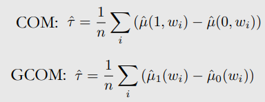
• COM은 1개의 NN을 사용
  • 모든 data에 fit한 model
• GCOM은 2개의 NN을 사용
  • T=1 network는 treatment group data로 trained
  • T=0 network는 control group data로 trained
  • networks는 higher variance를 갖게 됨 → not efficient

6-3. Increasing Data Efficiency

TARNet

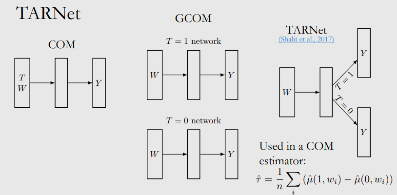
• COM은 biased
• GCOM은 high variance(너무 적은 data)
• TARNet은 treatment agnostic representation을 갖는 layer가 있다.
• inefficient
  • subnetwork가 group data로 학습되기 때문에

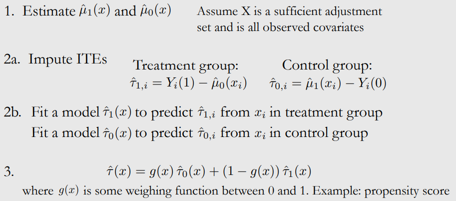
X-Learner

1. Estimate $\hat\mu_1(x)$, $\hat\mu_0(x)$ (X는 sufficient adjustment set, observed covariates)

2. Impute ITEs
   Treatment group : $\hat\tau_{1,i}=Y_i(1)-\hat\mu_0(x_i)$
   1개의 observed outcome in treatment group - potential outcome from all of the data in control group
   Control group : $\hat\tau_{0,i}=\hat\mu_1(x_i)-Y_i(0)$

3. $\hat\tau_{1}(x)$, $\hat\tau_{0}(x)$ 모델링

4. $\hat\tau(x) = g(x)\hat\tau_{0}(x) + (1-g(x))\hat\tau_{1}(x)$
   g(x)는 weighted function 0~1 → prpensity score

이해 안됨

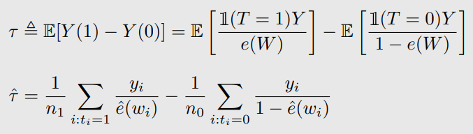
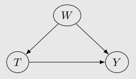
6-4. Propensity Scores and IPW

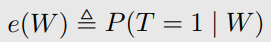
Propensity Score Theorem

positivity 일 때,
unconfoundedness given W → unconfoundedness given the propensity score e(W)
(W는 sufficient adjustment set)

• W가 high-dimensional이여도 e(W)는 1-dimensional
  
• 증명 : $P(T|W)=P(T=1|W)=e(W)$ (T가 binary라서)
  

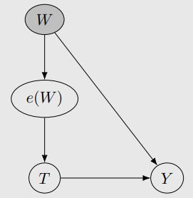
Positivity-Unconfoundedness Tradeoff에 적용

• overlap과 adjustment set의 dimension은 반비례하다
• 고차원의 W을 1차원으로 바꾼다.
• 하지만, propensity score에 접근할 수 없다. logistic regression과 같은 것으로 모델링할 수 있다.

잘 모름

6-5. Other Method

Pseudo-population

association == causation

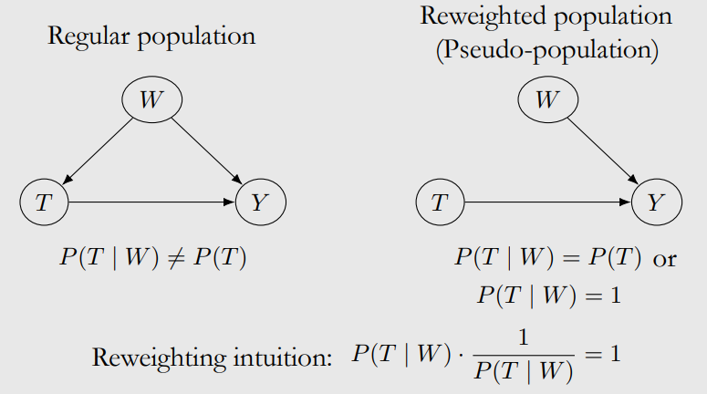
왜 1이 되면 끊어지지? T가 W에 independent해지지?

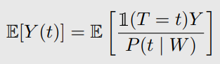
Inverse probability weighting(IPW) → COM

이해안됨.

$\hat{e}$로 propensity score approximate

이해안됨

효과가 줄어드나? 이해안됨.

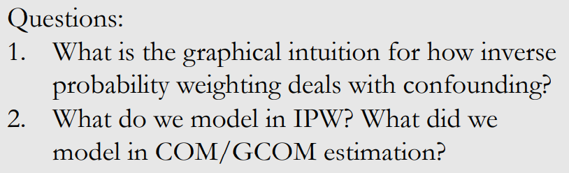
IPW CATE estimation

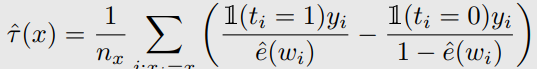
• natural 하지 않음
  값이 x인 것을 모아서 함.
  data point가 x인게 적다면 잘 안됨.

이해안됨.

Other methods

Conditional outcome models $\mu(t,w)$과 propensity score models e(w)을 사용

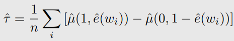
propensity score theorem을 통해 w를 condition을 하는 것 만큼 propensity score condition하는 것도 좋다.

Doubly robust methods

이해 못함.

Matching

roughly covariates가 비슷한 것끼리 match, match 안된 건 분석에서 제외

Double machine learning

• Stage1
  • W → Y의 모델 $\hat{Y}$
  • W → T의 모델 $\hat{T}$
• Stage2
  • $Y-\hat{Y}$ → $T-\hat{T}$의 모델로 W를 partial out

Causal trees and forests

• decision tree는 flexible하고, valid confidence intervals을 yield
• 그동안은 point estimate를 했다.
• 하지만 finite data로 uncertainty가 있음 → intervals를 놓는게 낫다.
• interval은 sampling variability를 encompass한다.