https://www.bradyneal.com/causal-inference-course
Introduction to Causal Inference라는 강의를 듣고 정리했습니다.

7. Unobserved Confounding, Bounds, and Sensitivity Analysis

7-1. Bounds

• unconfoundedness를 가정하면 point estimation이 가능
• weaker assumption을 사용하면 interval로 estimation (partial identification, set identification)

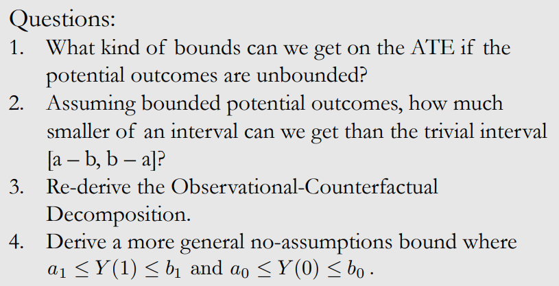
7-1-1. No-Assumptions Bound

Bounded Potential Outcomes

$-1\leq Y_i(1)-Y_i(0)\leq 1$
trivial length limit : 2

$a-b\leq Y_i(1)-Y_i(0)\leq b-a$
trivial length limit : 2(b-a)

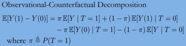
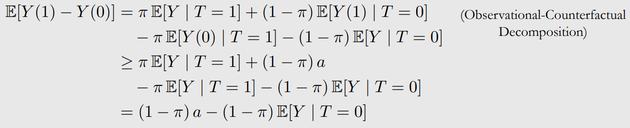
Observational-Counterfactual Decomposition

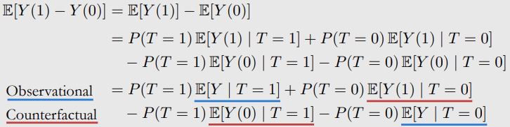
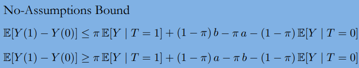
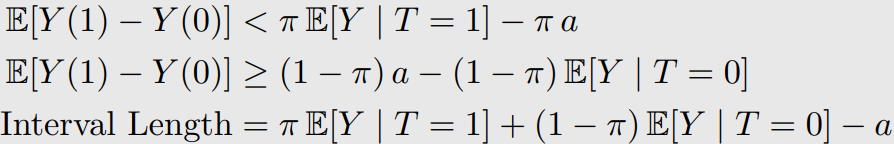
No-Assumptions Interval Length

$(1-\pi)b+\pi b -\pi a -(1-\pi)a=b-a$

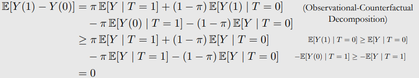
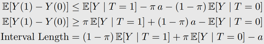
7-1-2. Monotone Treatment Response

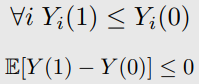
Nonnegative Monotone Treatment Response (MTR)

항상 treatment가 효과가 있을 때, $\forall i Y_i(1) \geq Y_i(0)$
ITE의 평균은 non-negative ($E[Y(1)-Y(0)]\geq 0)$)

• 증명
  

Nonpositive Monotone Treatment Response

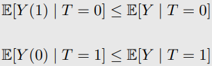
7-1-3. Monotone Treatment Selection (MTS)

• 가정 : 좋은 outcome을 내는 units은 treatment group으로 self selection된다.
  

• MTS
  

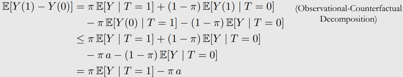
7-1-4. Optimal Treatment Selection

• 가정 : individual은 그들에게 도움되는 treatment를 항상 받게 되어있음
  

• OTS
  
  

• OTS Upper Bound 1
  

• OTS Lower Bound 1
  

• OTS Complete Bound 1
  

• OTS Complete Bound 2
  

• OTS Bound 1과 OTS Bound 2를 합쳐서 사용한다.

7-2. Sensitivity Analysis

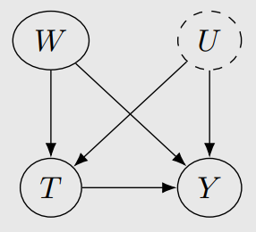
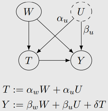
U가 unobserved confounder일 때,
U를 adjust하지 않은 거랑 실제 U를 adjust한 것과 얼마나 차이가 있는지를 분석하는 것이다.

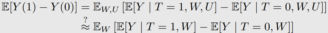
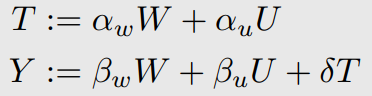
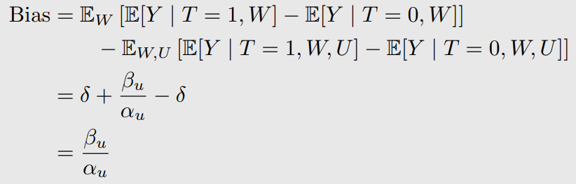
7-2-1. Linear Single Confounder

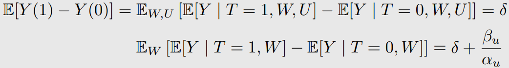
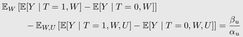
위와 같이 bias가 생긴다.

Contour Plots for Sensitivity to Confounding

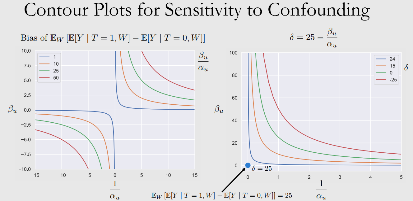
이해 안됨.

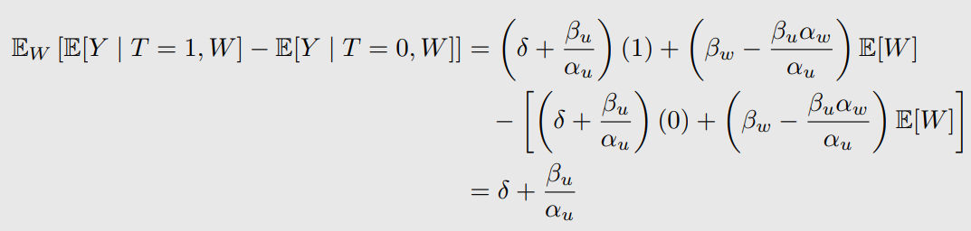
Bias in Simple Linear Setting 계산

Linear SCMs이 되면 이렇게 bias를 계산할 수 있다.
Linear이 아니면 방법이 없나?
여기서 bias의 의미가 뭐지?

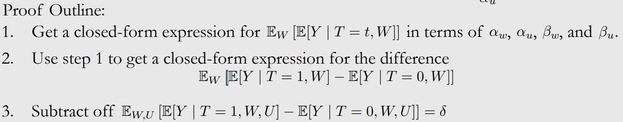
1. close-form expression 계산
   
   

2. 

3. 

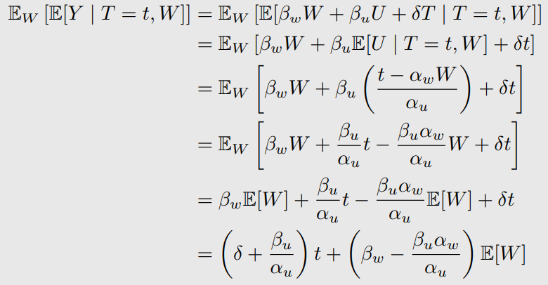
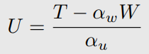
여기서 $\alpha_u, \beta_u$는 아래와 같다.

7-2-2. Towards More General Settings

위처럼 계산되는 것은 binary treatment일때

• T가 simple parametric form
• Y가 simple parametric form
• U가 binary, scalar