[ISLR] Chap 7. Moving Beyond Linearity

목표: 선형성 가정을 하지 않고도 해석이 가능한 모델 만들기

• Polynomial regression: 기존의 predictor의 power를 높이면서 선형 모델 확장
  • cubic regression: X, X^2, X^3
• Step function: 변수의 범위를 K개로 분리
• regression spline: 변수의 범위를 K개로 분리 + 그 범위 안에서 polynomial function 도입
  • region boundary에서 이 함수들이 smooth하게 이어질 수 있도록 함
• smoothing spline: regression spline과 비슷. RSS 값을 최소화하는 기준으로
• local regression: spline과 비슷하지만 region이 겹치는 것을 허용
• generalized additive model: multiple predictors

7.1 Polynomial Regression

• εi: 오차
• x, x^2, x^3...를 가지는 선형 회귀식
• 보통 d 값은 3, 4보다 크지 않음
  
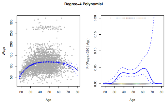
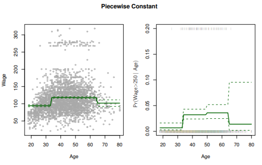
• Age와 Wage 간의 관계 확인을 위해서는 각각의 추정 계수 보다는 전체 적합된 함수에 초점
• 좌측 그래프를 보면 high earners, low earners로 나뉘어짐
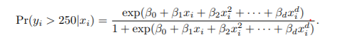
  • logistic regression으로 binary group 형성 가능
    
• 우측 그래프는 high earners에 대한 regression model
  • 전체 데이터 3000개 중 79개 뿐이라서 높은 분산과 넓은 confidence interval을 가짐

7.2 Step Functions

• polynomial function은 X에 대한 비선형 함수에 대한 전역 구조가 적용
• step function은 X의 범위를 bins로 나누어 각 bin에 다른 상수를 적합
  
• Ck는 indicator function
  
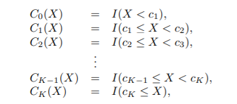
  • 이렇게 정의된 X를 dummy 변수라고도 함
  • 모든 Ck의 합은 1
    
• 각 bin 안에서의 trend를 놓칠 수 있음
  ex. first bin에서 increasing trend를 무시함

7.3 Basis Functions

• b1(x), b2(x),...에 대한 standard linear model
  • linear regression에 사용되는 모든 추정 tool(coefficient estimate, standard error, F-statistics) 사용 가능
• polynomial function: bk(x) = x^k
• piecewise constant function: bk(x) = I(ck≤x<ck+1)

7.4 Regression Splines

Piecewise Polynomials

• X의 region마다 low-degree polynomials 적합
• knots: coefficient가 변화하는 point를 knots
  • knots가 많아질수록 flexible한 모델
  • K개의 knots -> K+1개의 cubic polynomials
• ex.
  
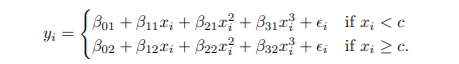
  • c: knots
  • 각각의 polynomial funtion은 least quares를 사용하여 fit

Constraints and Splines

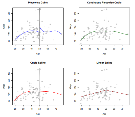
• piecewise cubic: X = 50 에서 연속이 아님
  • df: 8
• continuous piecewise cubic: X = 50 에서 연속
• cubic spline: X = 50 에서 연속, first derivative 연속, second derivative 연속
  • df: 5(=8-3(constraints))
  • 보통 4+K개의 df를 가짐(K=knots의 개수)
    • 두 점을 연결하는 선: 3차 다항식 -> df=4
    • knots 하나당 df=1 추가
• linear spline: X = 50 에서 연속

The Spline Basis Representation

Cubic spline

• X, X^2, X^3, h(X, ε1), ... , h(X, εk): K+3개의 predictors
• K+4개의 regression coefficients
• h(X, ε): truncated power basis
  

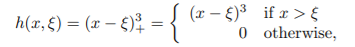
Natural spline

: 끝의 boundary에서는 함수가 linear하도록 boundary constraints가 추가된 spline

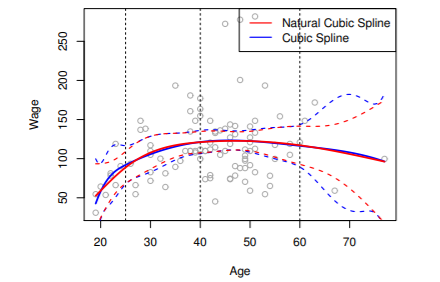
• cubic spline의 경우 가장자리 boundary에서 분산이 매우 큼
• natural spline을 사용해서 더 stable한 추정값을 얻을 수 있음

Choosing the Number and Locations of the Knots

Where should we place the knots?

• 함수가 가장 빠르게 변할 것 같은 곳에 많은 knots를, stable할 것 같은 곳에 적은 knots를 배치
• uniform 형태로. ex. 25, 50, 75 percentiles

How many knots should we use?

• 다양한 수의 spline 해보고 가장 좋아보일 때로 정함
• cross-validation을 통해 RSS가 가장 작아질 때로 정함

Comparison to Polynomial Regression

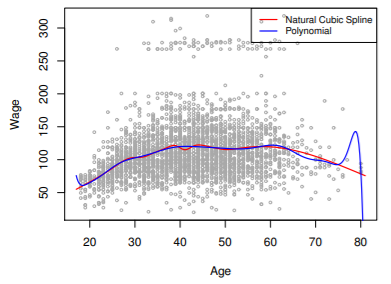
• regression spline이 더 좋은 결과
  • degree는 고정된 상태에서 knots의 개수만 증가시켜 flexibility 증가 -> 더 stable

7.5 Smoothing Splines

An Overview of Smoothing Splines

• smoothing spline: 위 식을 최소화하는 함수 g
• loss+penality 형태
  • loss function: encourages g to fit data well
  • penalty function: encourages g to be smooth
    • second derivative function(-> measures roughness)의 integral 형태: g가 smooth 하면 값이 작음
• λ: tuning parameter
  • λ=0: 과적합 가능성 높음
  • λ=무한대: linear least squares line
  • 편향-분산 트레이드오프 조정
• 위 식을 최소화하는 함수 g(x)는 knots를 x1~xn에서 가지는 natural cubic spline
  • shrunken version of natural cubic spline
  • λ 값이 shrinkage 값을 조정

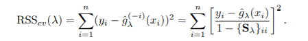
Choosing the Smoothing Parameter λ

• dfλ: measure of flexibility of the smoothing spline
• fitted values of g
  
  • Sλ: nxn matrix
  • y: response vector
• effective degrees of freedom: Sλ의 대각 요소의 합
  
• LOOCV(leave-one-out CV)를 통해 계산된 RSS가 가장 작을 때의 λ 선택
  
• ex.
  
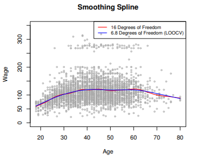
  • 두 경우 차이가 크지 않으므로 이 경우에는 비교적 간단한 모델인 6.8 df spline을 선택

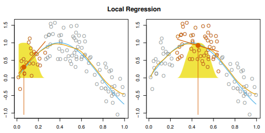
7.6 Local Regression

: target point에서 이웃 데이터만을 가지고 fit

과정

Step 1: x0와 가까운 s = k/n만큼의 학습데이터를 선택

• span s에 따라 flexibility가 변함
• s가 커지면 global fit이 됨

Step 2: Ki0 = K(xi, x0) 을 각 point에 지정

• x0와 가장 먼 point의 weight = 0

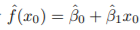
Step 3: wls 학습

• 위 식을 최소화하는 β0, β1 찾기

Step 4: fitted value

• ex.
  

varying coefficient model의 적용

• 최근에 수집된 다양한 계수 모형 데이터에 모형을 적용하는 경우에 유용
• 변수 X1과 X2 쌍에 로컬인 모형을 적합하려는 경우에 유용
• 하지만, 차원이 3, 4 이상으로 높아지면 결과가 안 좋음(b/c x0에 가까운 훈련 데이터셋이 적음)

7.7 GAM(Generalized Additive Models)

• 다중 선형 회귀의 확장(변수 여러 개)
• additivity를 유지하면서 각 변수의 비선형 함수로 확장

GAMs for Regression Problem

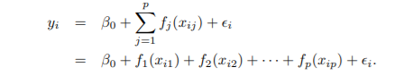
• multiple regression에서 βjXij를 fj(xij)로 대체한 형태
• why additive model?
  • Xj에 대해 개별 fj를 계산하여 그들을 합한 것으로 나타내었기 때문
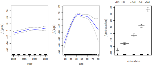
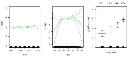
• ex.
  
  • f1, f2: natural splines, f3: step function(dummy variable)
    
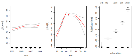
    • least square 방법으로 fitted value 구할 수 있음
    • 다른 변수들을 고정시켜두었을 때,
      • year에 따라 wage 증가
      • intermediate age일 때 wage가 최고
      • education에 따라 wage 증가
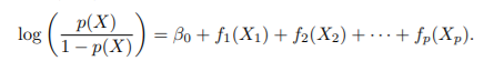
  • f1, f2: smoothing splines, f3: step function(dummy variable)
    
    • gam()이라는 함수가 backfitting 방법을 통해 계산
    • backfitting: 다른 변수들은 고정시킨 채로 변수마다 돌아가면서 fit을 update하는 방식
• 보통은 natural spline과 smoothing spline을 섰을 때의 차이가 작음
• 다른 모델을 사용해도 됨(local regression, polynomial...)

GAMs for Classification Problem

• 마찬가지로, 로지스틱 회귀의 식에서 βjXij를 fj(xij)로 대체한 모델
• ex.
  
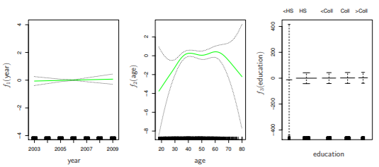
• education에서 맨 왼쪽 변수의 CI가 매우 큼 -> 데이터 상으로 이에 해당하는 wage가 250이 넘는 사람이 없음 -> 삭제
  
• high earner에게는 age와 education이 year보다 큰 영향이 있음

Pros and Cons of GAMs

Pros

• Xj에 대해 비선형 fj를 fit하기 때문에 선형 회귀가 놓칠 비선형 관계까지 자동으로 모델링할 수 있음
• Y에 대한 더 정확한 예측이 가능
• additive model이기 때문에 각 Xj의 Y에 대한 영향을 개별적으로 확인 가능
• fj의 smoothness는 자유도로 설명 가능

Cons

• additive에 제한됨
• 중요한 interaction을 놓칠 수 있음
• But, 선형 회귀처럼 interaction term을 추가할 수 있음