Following the previous post, I will introduce the "Classifier-Free Diffusion Guidance" paper.

I presume that you have known the previous paper "Diffusion Models Beat GANs on Image Synthesis". If you do not know this paper well, you should refer to this post: https://velog.io/@yhyj1001/Diffusion-Models-Beat-GANs-on-Image-Synthesis.

I will call the name of the previous paper's method "ADM-G," which means "Ablated Diffusion Model-Guidance."

Motivations & Contributions ⭐️

Motivations 📚

• ADM-G has needed an auxiliary classifier model $q_\phi (c|x_t)$. This means that we have to pre-train this classifier with decayed data $x_t$. Resultantly, this has caused a complex training pipeline.
• Inception Score (IS) and Frechet Inception Distance (FID) are computed using the classifier model, the Inception model. Authors contend that classifier-guided diffusion sampling can be understood as an effort to perturb an image classifier using a gradient-based adversarial attack to create confusion because this method employs both a score estimate and a gradient of the classifier model.

Contributions ⭐️

• Authors propose a classifier-free diffusion guidance.
• They show that diffusion models are able to trade off diversity for fidelity without an auxiliary classifier.

Methods

Classifier Guidance

In the previous post, we defined a conditional reverse process with a scale factor $w$.
In this paper, authors use the SNR parameter $\lambda$ because they define the continuous variance-preserving diffusion process.

First of all, they derive a conditional reverse process as the above equation. According to the previous paper, $\epsilon_\theta(x_t) = {1\over \sigma_\lambda}\nabla_{x_\lambda}\log p(z_\lambda | c)$ is satisfied. In addition, the reason why this term is defined with $p(z_\lambda | c)$ is that the model gains the conditional factor using the AdaGN module.

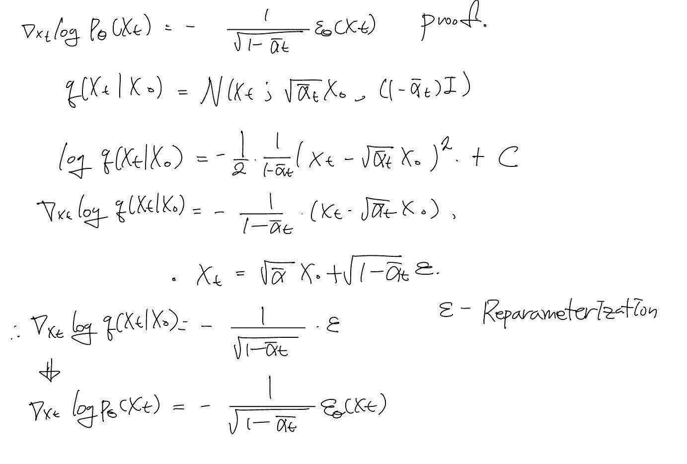
Resultantly, authors can represent the above term when $\tilde \epsilon_\theta(z_\lambda, c) = -\sigma_\lambda \nabla_{z_\lambda}\log \tilde p_\theta(z_\lambda|c)$. (Proof 1)

Classifier-Free Guidance

In this section, the authors propose the classifier-free guidance method for a conditional reverse process.

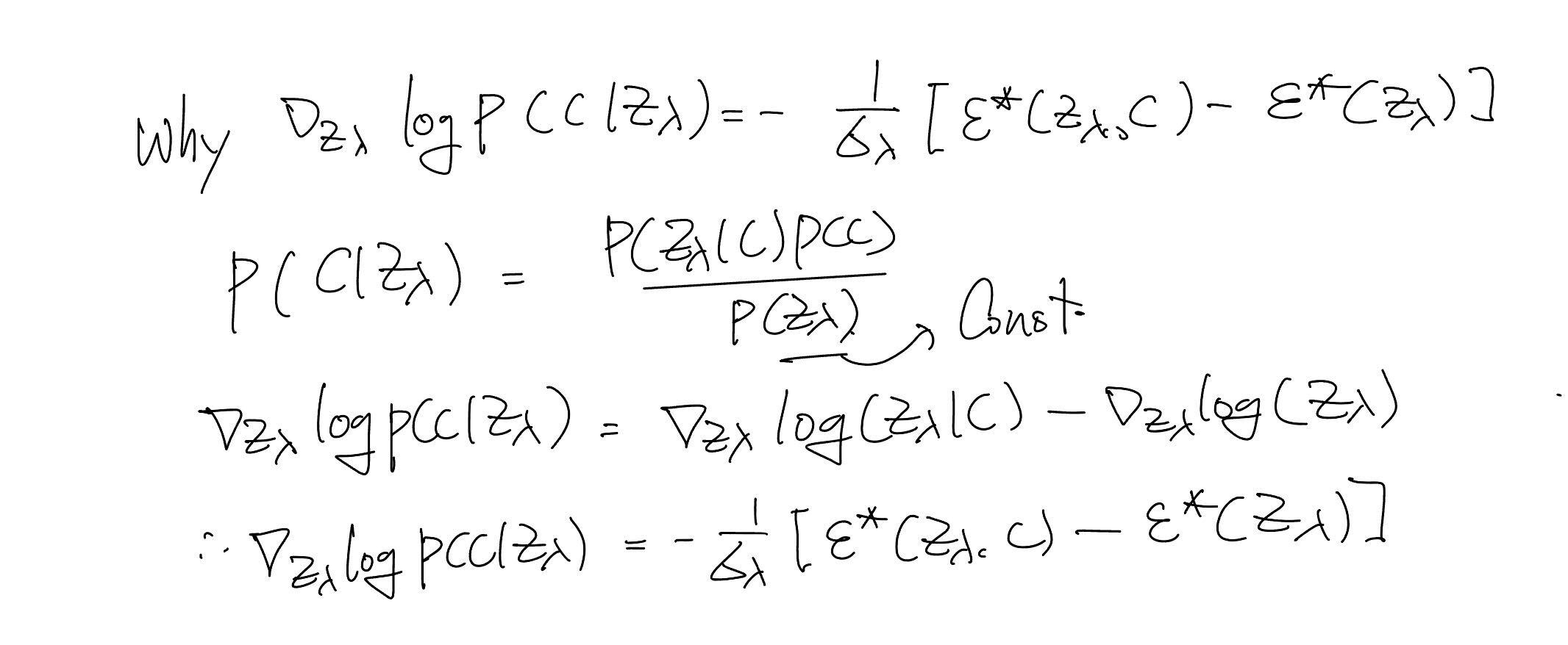
They were inspired by the gradient of the implicit classifier definition: (Proof 2)

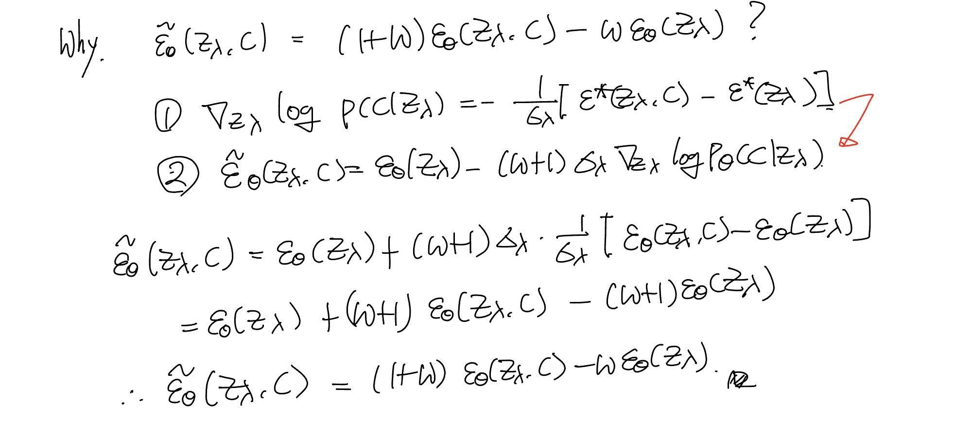
By the above definition, they derive the linear combination of the conditional and unconditional score estimates:

The above term can be derived using all equations in this post. (Proof 3)

In fact, the term (Proof 2) assumes that the score estimate should be the optimal value. However, the authors claim that they empirically found that the non-optimal term has performed well, even if naively defined.

Based on the above definition, they illustrate the classifier-free guidance algorithm:

Results

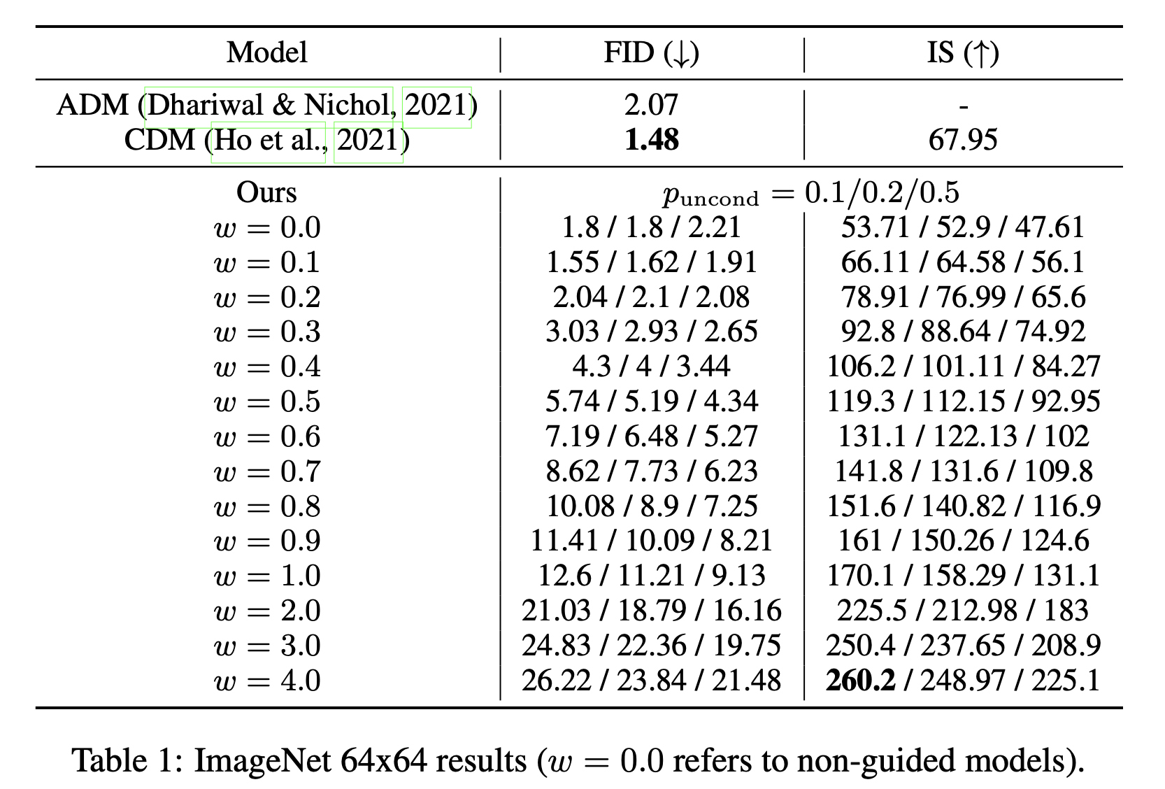
They prove that the classifier-free guidance method can trade off diversity for fidelity with the scale factor and the unconditional training probability. As the above table shows, they can achieve the best fidelity but poor diversity when using the lowest unconditional training probability and the highest scale factor (high FID value / high IS value).

Proof / Appendix

1.

2.

3