Generative Modeling by Estimating Gradients of the Data Distribution (1) - A Connection Between Score Matching & Denoising Autoencoders

Seow·2024년 7월 5일

Diffusion

목록 보기

6/8

In this post, I will introduce denoising score matching. We have to define some mathematical proofs in order to comprehend the connection between score matching and denoising autoencoders.

In short, I am going to explain some underlying knowledge for understanding NCSN (Noise Conditional Score Network).

GOAL 🎯

Relationship between Denoising AutoEncoder (DAE) and Score matching.

Parzen Kernel Estimation

Authors employ a parzen window in order to define some theorems quite strictly. Thus, I'm going to explain about this.

Parzen window is a simple concept for density estimation. In the paper, authors apply this concept to define expectations with probability density function, $q_\sigma (\tilde x)$ .

Parzen density estimation is defined with hyper-cube; Parzen window :

K = \Sigma^N_{n=1} k(x-x_n)\\[8pt] k(u) = \begin{cases} 1 & \text{if} \; |u_i|>{1\over2}h~~i=\{1,2,...,D\}, \\ 0 & \text{else}. \end{cases}\\[8pt] p(x) \approx {K\over NV}

In the above equation, N and K are the total amount of data and the number of data in the Parzen window, respectively. V and k are the volume of the Parzen window and the Parzen window, respectively.

Linear / Tied weights DAE

In the paper, they try to define the connection between score matching and denoising autoencoder. Therefore, I will introduce a Denoising Autoencoder (DAE).

As you can know by the name "DAE", this is a simple autoencoder trained with noisy input and clear ground truth. In this paper, the authors assume that the encoder and decoder are composed of a linear weight and are shared. Resultantly, the objective of this model can be defined as :

J_{\text{DAE}_{\sigma}}(\theta) = \mathbb{E}_{q_\sigma(\tilde x, x)} [||W^{T}\text{sigmoid}(W^T\tilde x + b)+c - x||^2]

Explicit Score Matching

Notations

$p(x;\theta)$ : probability density model
$p(x;\theta)={1\over Z(\theta)}\exp (-E(x;\theta))$
$E(x;\theta)$ : energy function

Langevin Sampling Method

In this section, I do not deal with the Metropolis-adjusted Langevin Algorithm.

First of all, I introduce "overdamped Langevin Ito diffusion".
This is defined as $\dot X = \nabla \log p(X) + \sqrt 2 \dot W$ . In this definition, $\dot W$
is a Brownian motion. This means that the equation is a Markov chain and a stochastic process. In addition, a probability distribution of $X(t)$ would be $p(X)$ when $t\rightarrow\infin$ .

In order to use this method, we have to discretize this definition. Simply, we just apply Euler-Maruyama method.

X_{t+1}= X_t + \tau \nabla \log p(X) + \sqrt {2\tau} z ~, ~z\sim N(0, I)

ESM : Explicit Score Matching

A probability function can be expressed as $p(x;\theta)={1\over Z(\theta)}\exp (-E(x;\theta))$ . In the expression, $Z(\theta)$ requires high computational costs. Therefore, we need indirect methods in order to understand $p(x;\theta)$ . The score-matching method is one of these methods.
Original score functions are defined as $\partial \log p(x;\theta)\over \partial \theta$ , but the explicit score functions in this paper are defined as :

\phi(x;\theta) = {\partial \log p(x;\theta)\over \partial x}

If we can model this function well, we can generate clear samples using the Langevin sampling method. This is because score functions mean a gradient flow of log probability density. Thus, we can perform a gradient ascent of probability density through the Langevin sampling method.

In order to train the score function, the objective can be defined as:

J_{ESM_{q}} = \mathbb{E}_{q(x)}[{1\over2}||\psi(X;\theta) - {\partial \log q(x)\over \partial x}||^2]

However, we cannot know $q(x)$ ... Therefore, we have to find other methods to model the score function.

Implicit Score Matching

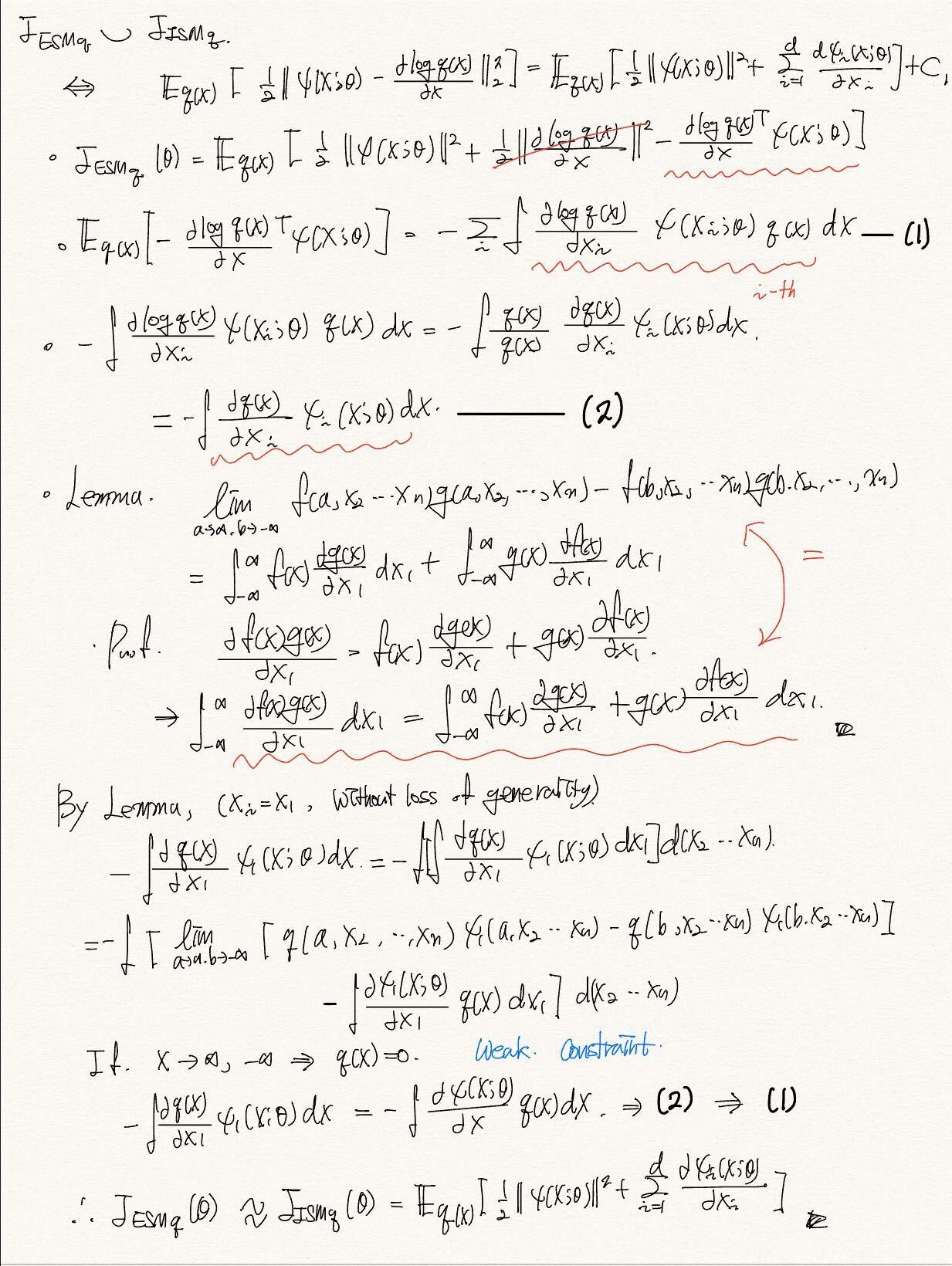
Make a long story short, Implicit Score Matching (ISM) is a method to train score functions, and the objective is defined as:

J_{ISM_q} = \mathbb{E}_q[{1\over 2}||\psi(x;\theta)||^2+\sum^d_{i=1}{\partial \psi_i(x;\theta)\over \partial x_i}]

So, how can this term be derived? The details are in [Estimation of Non-Normalized Statistical Models by Score Matching : Theorem 1]. In this paper, authors prove that $J_{ESM_q} \smile J_{ISM_q}$ if some weak constraints are satisfied. $J_{ESM_q} \smile J_{ISM_q}$ means that these objectives result in same outcomes.

Proof:

In this proof, the last line has wrong sign. It must be $-\int {\partial q(x)\over \partial x}\psi(x;\theta) dx = \int {\partial \psi(x;\theta)\over \partial x} q(x) dx$ .

Matching the Score of a Non-Parametric Estimator

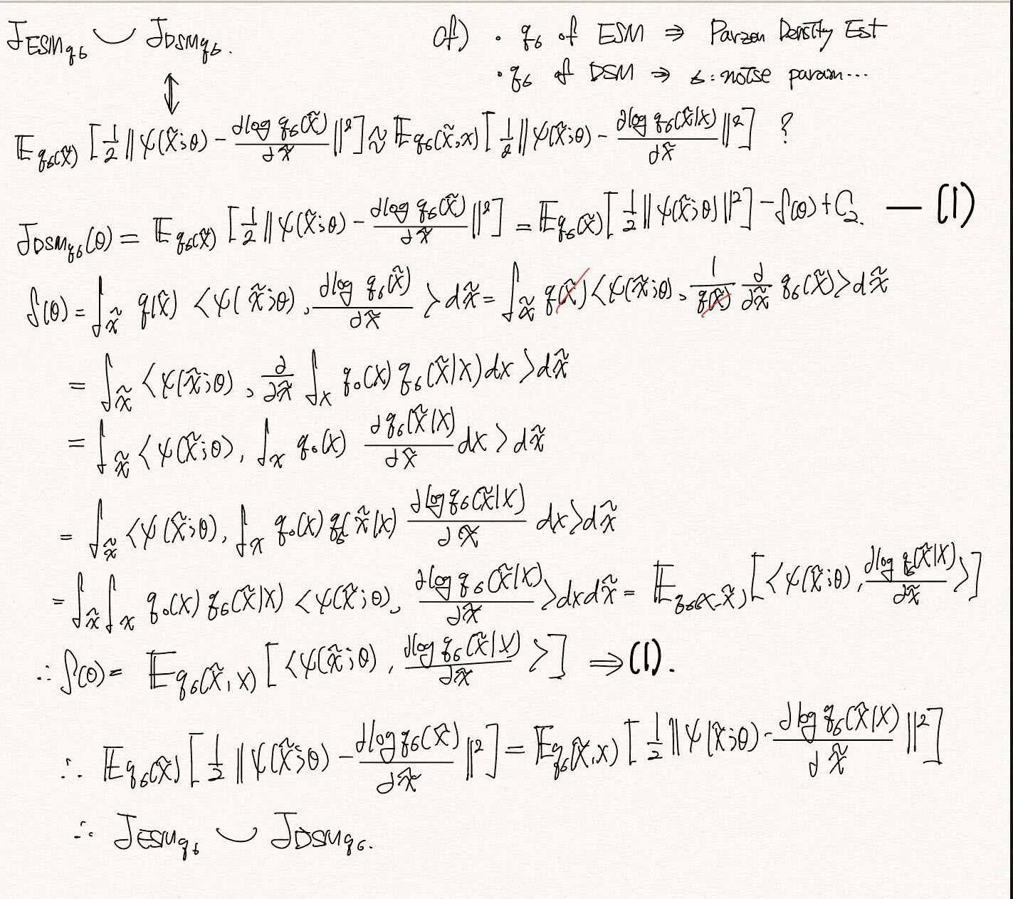
The above definition can be expressed using a non-parametric Estimator, a Parzen window. Let's define $q_\sigma(\hat x)$ as a non-parametric estimator with a Parzen window (hyper-cube) which has a $\sigma$ hyperparameter. Even if we define the ESM and ISM with the non-parametric estimator, the equality is satisfied.

J_{ESM_{q_\sigma}} \smile J_{ISM_{q_\sigma}}

Denoising Score Matching

First of all, ISM has a critical disadvantage. They require expensive computations because the objective of ISM needs the Hessian of the given model.

To alleviate this proble, we can use the Denoising Score Matching (DSM).

J_{DSM_{q_\sigma}}(\theta) = \mathbb{E}_{q_\sigma(x, \tilde x)} [{1\over2}||\psi(\tilde x; \theta) - {\partial \log q_\sigma(\tilde x | x)\over \partial \tilde x}||^2]

In this equation, ${\partial \log q_\sigma(\tilde x | x)\over \partial \tilde x}$ is tractable because $q_\sigma(\tilde x | x)$ is a Gaussian distribution. Therefore, we can directly calculate the score function.

Proof : Appendix in the technical report : A Connection Between Score Matching and Denoising Autoencoders

https://www.iro.umontreal.ca/~vincentp/Publications/smdae_techreport.pdf

Proof:

이게 왜 작동하는가? -> proof에서 parzen density estimator를 기반으로 전개된 ESM과 비교하여 동일하다는것을 보인다. parzen density estimator와 real sample에 대한 random variables를 가지고 marginalization technique을 써서 전개를 해 나가는데, 이게 noise가 더해진 noisy data를 사용하는 것과 비교하는데 어떻게 이론적으로 맞는지가 잘 와닿지 않는다.
하지만 parzen estimator와 같은 estimator와 noisy한 샘플에 대한 pdf를 같게 볼 수 있지 않을까 라는 생각이 들긴 한다. 사실 Expectation을 사용하는 것 자체가 noise의 영향을 어느정도 배제할 수 있기 때문에 Expectation에 noised data 에 대한 데이터분포를 고려하는 것 자체가 estimator처럼 작동할 수 있었던것 아닐까.

Seow

이전 포스트