Today, I will introduce well-known paper "Diffusion Models Beat GANs on Image Synthesis."
When this paper was introduced, many people were startled because the diffusion model first completely eclipsed the GAN-based model, Big-GAN.
I do not explain the rigorous formula of a diffusion process in this post. If you do not know about this, check these posts.
- DPM : https://velog.io/@yhyj1001/DPM-Deep-Unsupervised-Learning-using-Nonequilibrium-Thermodynamics
- DDPM : https://velog.io/@yhyj1001/DDPM-Denoising-Diffusion-Probabilistic-Models
- Lil'Log diffusion process : https://lilianweng.github.io/posts/2021-07-11-diffusion-models/
Motivations & Contributions ⭐️
Motivations 📚
- Authors explore that the reason why diffusion models could not surpass GAN-based models for image fidelity.
- First, GAN architecture has been improved for a long time.
- Second, GAN-based models are able to trade off diversity for fidelity.
Contributions ⭐️
- Authors explore and construct an effective model architecture through ablations.
- They also propose a classifier-guidance method in order to achieve the ability to trade off diversity for fidelity.
Methods
Architecture Improvements
They perform several architectural ablations to find the architecture that achieves a conspicuous performance.
They explore several architecture changes like the number of attention heads, diverse resolutions of attention, employing residual blocks, and so on.
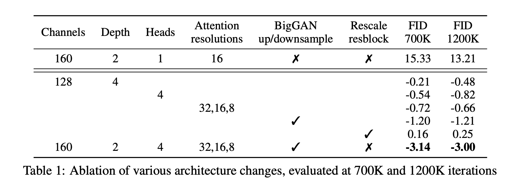

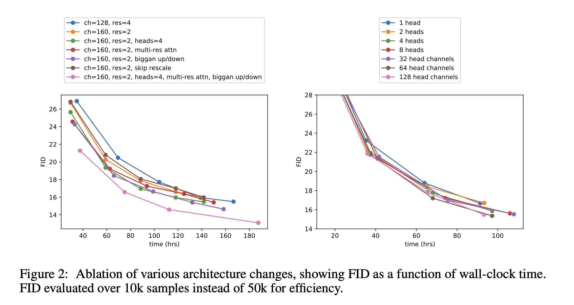
In accordance with above experimental results, they determine the final model: 2 residual block / 2 multiple heads with 64dim per head / attention at 32, 16 and 8 resolutions / employing BigGAN residual blocks for up and downsampling.
In addition, they experiment with adaptive group normalization (AdaGN). This module can incorporate the timestep and class embedding into each residual block after a group normalization.

They find that the AdaGN module achieves better performance than the simple conditioning method (Addition + GroupNorm).
Resultantly, they also employ the AdaGN modules.
Classifier Guidance
According to authors' claim, an ability to trade off diversity for fidelity is a reason why GAN-based models can achieve superior performance than diffusion-based models. This means that GAN-models can generate high quality samples but not cover the whole data space.
Therefore, they try to incorporate class information with a classifier .
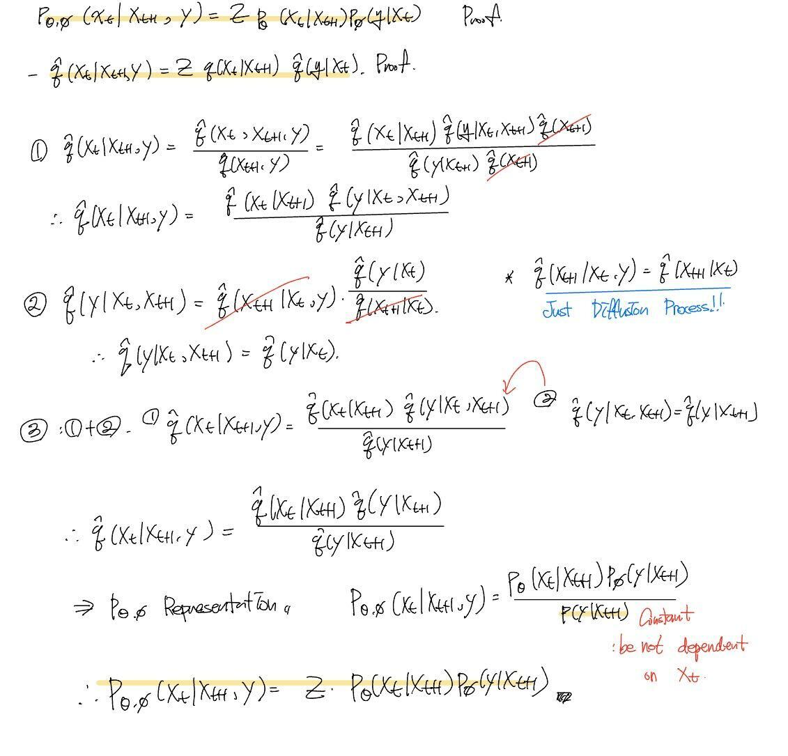
First of all, they define a reverse process guided by a classifier. (Proof 1)
The above multiplication term can be divided with log transformation. Thus, we should consider each term.
The first term is a unconditional reverse process. So, this term can be represented as the Gaussian distribution . If we transform this term through log transformation, this term is :
The second term is a classfier, and we can approximate using a Taylor expansion around . This is because we can presume that has relatively low curvature compared to . (As you know, diffusion process assume that it has infinte diffusion steps. Thus, .)


According to this fact, we can derive the above equation.

As a result, we can conduct the classifier guided diffusion sampling through the above algorithm.
Conditional Sampling for DDIM
In DDIM, they assume that there is no randomness between the adjacent timestep states. Therefore, the sampling method proposed in the above section cannot be used.
To find a conditional sampling method in this setting, authors use a score-based conditioning trick [1]. [1] proposed continuous-time diffusion process using SDE. According to the paper, the conditional reverse process is defined as:

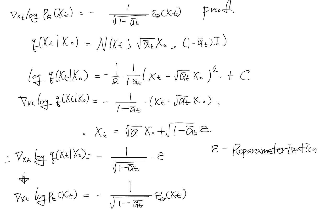
Thus, authors try to represent term as a score function like the below equation. (Proof 2)
By this form, they define the conditional reverse process.

Resultantly, they can derive the below conditional term.


The overall algorithm of this method is illustrated in the above figure.
Scaling Classifier Gradients
Authors found it necessary to scale the classifier gradients by a constant factor larger than 1. This is because they observed that the classifier assigned reasonable probabilities (about 50%) to the desired classes for the samples, but the samples did not match the intended classes upon visual inspection.
They found that scaling up the classifier gradients could alleviate this problem.

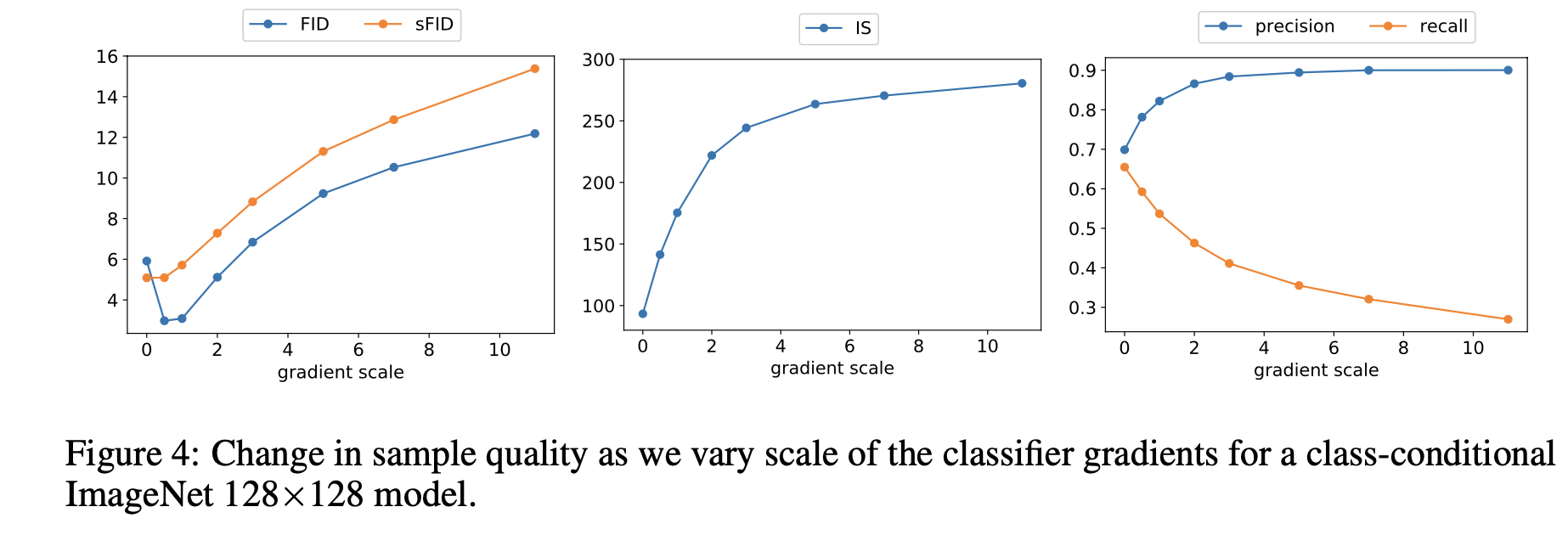
As the above figures illustrate, when the scale value is large, diversity is heightened, but fidelity is lowered (Precision / Recall).
Results
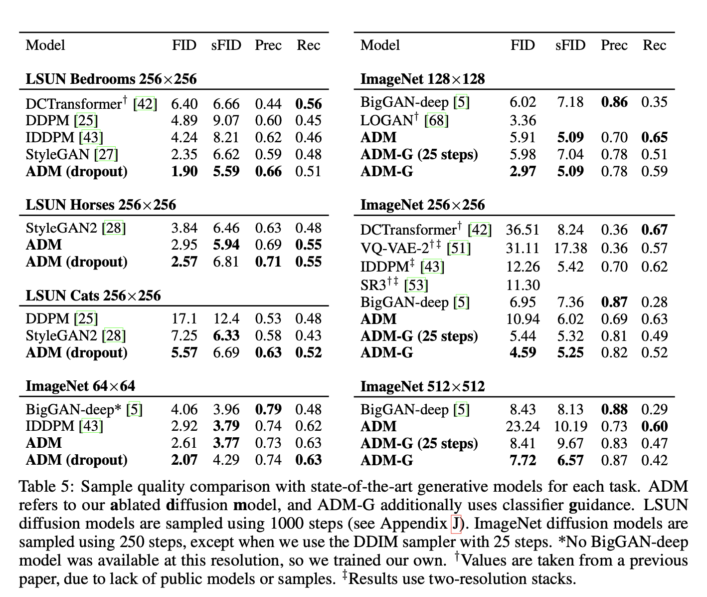
STATE-OF-THE-ART IMAGE SYNTHESIS
Reference
[1] Song, Yang, et al. "Score-based generative modeling through stochastic differential equations." arXiv preprint arXiv:2011.13456 (2020).
Proof / Appendix
1.
2
