In this post, I'm going to introduce a paper named "Denoising Diffusion Implicit Models."

In the paper, authors get used to abuse 'joint / marginal' term. The joint and marginals means $q(x_{1:T}|x_0)$ and $q(x_t|x_0)$, respectively.

Motivations & Intuitions ⭐️

Motivations 📚

1. In the previous study, DDPM, the forward and reverse processes needed a myriad of steps because they were inspired by thermodynamics defined by continuous time.
2. Also, according to DPM paper, for both Gaussian and binomial diffusion, for continuous diffusion (limit of small step size β) the reversal of the diffusion process has the identical functional form as the forward process.
3. The Markov chain process is only dependent on an adjacent time step. Therefore, for stable systems, the process should be defined by a small interval.

Intuitions 🧐

1. Inspired by DDPM paper, authors try to generalize the processes by non-Markovian processes. (Joint distribution $q_\sigma(x_{1:T}|x_0)$ can be described in various ways.)
2. For generalization, they only define $q_\sigma(x_t|x_0)$ and $\alpha$ (decreasing sequence). This idea is based on the fact that the loss of DDPM is only dependent on $q(x_t|x_0)$.
3. These new processes are not diffusion processes anymore. $\rightarrow$ These processes don't have to be conducted with a myriad of steps.
4. The non-Markovian processes are dependent on both an adjacent sample $x_{t}$ and a clean sample $x_0$. Thus, there is more enough information for new sample $x_{t-1}$ than the Markovian process. (Personal theory)

Contributions ⭐️

1. Authors generalize the forward diffusion process used by DDPMs to non-Markovian ones.
2. Generalized train loss is the same as DDPM's train loss.
3. Superior sample quality (when accelerating sampling by 10$\times$ ~)
4. Consistency

Methods

Generalization of forward diffusion process

In this paper, the authors only define two conditions for achieving generalized results.

1. $q_\sigma(x_t|x_0)=\mathcal{N}(x_t; \sqrt{\alpha_t}x_0, (1-\alpha_t)\mathrm{I})~\mathrm{for~all}~t$
2. $\alpha_t$ is a decreasing sequence.

These conditions are derived from DDPM expressions.

Variational Inference for Non-Markovian Forward Processes

According to DDPM and other related papers, we can set the objective as the above form. $\gamma = [\gamma_1, ..., \gamma_T]$ is a vector of positive coefficients.

Due to the reparameterization in DDPM, the objective only depends on the marginals $q_(x_t|x_0)$, but no directly on the joint $q(x_{1:T}|x_0)$. If properties of probability are satisfied, any graphical models can be constructed. Therefore, the authors construct new graphical models using the non-Markovian process, which allows for inference in fewer timesteps. (the above figure.)
By defining the process like this, the newly defined one is not a diffusion process anymore, so it doesn't follow the principle, for continuous diffusion (limit of small step size β) the reversal of the diffusion process has the identical functional form as the forward process.

Non-Markovian Forward Process

First, they define the graphical model of the diffusion process, like the above equation. This definition allows the current timestep sample to depend on an adjacent sample and a clean example.

$q_\sigma(x_{t-1}|x_t, x_0)$ is a posterior of the forward process. This term can be derived to Gaussian distribution using the Condition 1. (eq 7)

In the above equation, $\sigma_t$ represents the how stochastic the forward process is. In DDPM, $\sigma$ is dependent on $\alpha$, but the authors do not define any relationship in this study. If $\sigma=0$, then the reverse process is deterministic given $x_t, x_0$.

"$\sigma_t$ represents the how stochastic the forward process is."
여기에서의 forward process는 $x_0$과 $x_t$가 주어졌을때 $x_{t-1}$이 어떻게 나올 것인지에 대한 posterior를 가지고 있는 forward process.

이 부분에서 왜 저자가 $q_\sigma(x_{t-1}|x_t, x_0)$ 형태의 posterior를 사용해서 non-Markovian process로 정의했는지 감이 온다. 본 연구에서 직접적으로 원하는 것은 reverse process에서 deterministic한 process를 정의하는게 목적이라 처음부터 이에 대해 고려해주기 위해 reverse process와 매칭되는 posterior로 명시한게 아닌가 싶다.

In order to derive the forward process in the non-Markovian process, they use Bayes' rule like the above term.

위의 정의된 non-Markovian process의 randomness는 두개의 path로 이루어져 있다.
1. 인접한 timestep 간의 관계
2. 0 -> t
현재의 상황에서는 $\sigma, \alpha$ 사이의 어떤 관계도 정의되어있지 않기 때문에 독립적인 path로 바라보는게 좋을듯 한다.

Generative Process and Unified Variational Inference Objective

In order to train the model, they define a trainable generative process $p_\theta(x_{0:T})$.
As we discussed, according to the non-Markovian process, we know that $p^{(t)}_\theta(x_{t-1}|x_{t})$ leverage knowledge of $q_\sigma(x_{t-1}|x_t, x_0)$.

위 learnable transition kernel을 $p^{(t)}_\theta(x_{t-1}|x_{t})$ 와 같이 (t)라는 superscript로 표현하는데, 이는 time t마다 독립적인 모델임을 암시한다 (weight가 공유되지 않음). 실제로 모델은 time t를 input data로 받고, 이는 time t에 대한 subspace의 훈련을 의미할 수 있다.
-> 근데 나에게는 다소 naive한 전개처럼 다가온다. time t를 input으로 넣는다고 해서 서로의 영향이 미치지 않는걸 보장할 수 있는가?

Corresponding the defined non-Markovian process $q_\sigma(x_{t-1}|x_t, x_0)$, inference process is conducted.

1. $x_t$ is given (current time step)
2. $x_0$ is derived with $x_t$ and definition of "the denoised observation", $f_\theta^{(t)}$.
   $f_\theta^{(t)}(x_t)=(x_t-\sqrt{1-\alpha_t}\cdot\epsilon_\theta^{(t)}(x_t))/\sqrt{\alpha_t}$
3. $x_{t-1}$ is derived with $x_t, x_0$ using $q_\sigma(x_{t-1}|x_t, x_0)$. (the below equation)
   

By these methods, the model is optimized with the following variational inference objective (eq11).

The above objective function is slightly different with $L_1$ (Simple ddpm loss). However, the authors found that the two objectives are same in some conditions.

First of all, they set the above theorem (the proof is in Appendix). As I stressed, they consider the models independent with timesteps $t$. In this situation, the model $\epsilon_\theta$ will not depend on the weights $\gamma$. Therefore, since $J_\sigma$ is equivalent to some $L_\gamma$ from Theorem 1, the optimal solution of $J_\sigma$ is also the same as that of $L_1$.

Sampling from Generalized Generative Processes

Denoising Diffusion Implicit Models

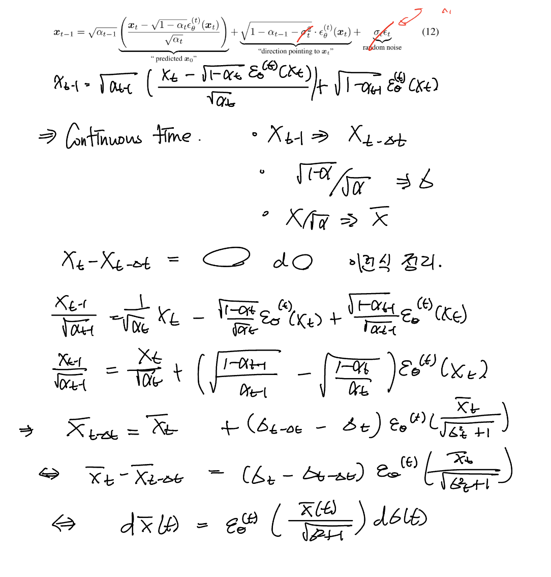
Basically, sampling can be conducted with $p^{(t)}_\theta(x_{t-1}|x_t)$ (Ancestral sampling or forward sampling). In accordance with the equation, the sampling process can be expressed as the above term, eq(12). When $\sigma_t = \sqrt{(1-\alpha_{t-1}/(1-\alpha_t))}\sqrt{1-\alpha_t/\alpha_{t-1}}$ for all $t$, the forward process is Markovian process, and overall processes become DDPM processes.

If $\sigma =0$, there is no randomness in the process, being the denoising diffusion implicit process (DDIM).

Accelerated Generation Processes

1. The loss $L_1$ is only dependent on the condition $q_\sigma(x_0|x_t)$.
2. We can manipulate the sampling process without modifying the loss.
3. Define the forward process, which does not consider all the latent variables $x_{1:T}$. -> only subset $\{\tau_1, \tau_2, ... ,\tau_S\}$.

By these processes, we can significantly reduce the timestep for sampling.

Relevance to Neural ODEs

이 논문에서의 ODE form은 process의 randomness를 담당하는 $\sigma$를 없앴기 때문에 자연스럽게 유도가 되지만, SDE-Diffusion에서의 ODE form은 SDE와 동일한 marginal probability density $p_t(x)$ 를 공유하는 deterministic path가 있다는 데에서 시작한다 (fokker-planck equation). 이 차이를 알아두면 좋을듯..

DDIM defined with $\sigma=0$ can be expressed as ordinary differential equations.

$\sigma$ in the equation is not the same term as eq(7).

Being able to define ODE means that the reverse of the generation process can be derived with enough discretization steps. Also, this suggests that encodings of the observations can be used. This is very useful for other downstream tasks.

VESDE (SDE-diffusion)와 DDIM의 ODE는 optimal model $\epsilon^{(t)}_\theta$에 대해 equivalent probability flow를 갖는다고 한다. 이에 대해서는 이해가 잘 가지 않는다. 왜 이해가 가지 않는지 이유를 기술해보고자 한다.

1. probability flow라는 말을 사용해도 되는가? - SDE diffusion 논문에서 probability flow (PF) ODE라고 부르는 이유는 SDE의 probability flow (time t에 따라 probability가 어떻게 변하는지)를 표현할 수 있는 fokker-planck equation으로 유도되기 때문인데, DDIM의 ODE는 이를 기반으로 풀어내는게 아니라 단순히 process가 deterministic하다는 성질을 통해 단순 수식 전개로 유도된다.

2. Appendix B 에서 VESDE의 ODE를 현재 form과 매칭되게 전개한다. 근데 VESDE는 NCSN(SMLD) 프로세스를 전신으로 하고 있기 때문에 $\sigma^2$는 $x_0 \rightarrow x_t$ process에 대한 variance가 된다 (geometric sequence). 근데 $\bar x(t) = \bar x(t) + \sigma(t)\epsilon$이라고 정의한다. 뭔가 여기에서부터 이해가 잘 가지 않는다.

3. $\sigma(t)$-perturbed score function $\nabla_{\bar x}\log p_t(\bar x) = \argmin_{g_t}\mathbb{E}[||g_t(\bar x) + \epsilon/\sigma(t)||^2_2]$은 이와 같은 minimizer 라고 한다. 어디에서 근거를 얻은건지 모르겠다 ((Vincent, 2011) 이 논문이라고는 한다.)

4. 위의 식 (13), (14)를 보면 원래 DDIM의 식에서 $\alpha, x_t$를 $\sigma, \bar x_t$로 재 정의 한다. 근데, appendix에서는 VE SDE의 식을 정리할때 애초에 $\sigma, \bar x_t$로 처음부터 정의한다. 변수들이라 괜찮을 것 같긴 하지만 엄연히 두 식에서의 $\sigma, \bar x_t$는 의미하는 바가 다르다. VE SDE에서는 geometric sequence $\sigma$와 process의 state라 볼 수 있는 $\hat x_t$이지만 DDIM에서 유도할때의 식에서는 $\bar x$는 random variable에 어떤 schedule에 속하는 scalar로 뺀거고, $\sigma=(\sqrt{1-\alpha}/\sqrt\alpha)$라서 geometric sequence와는 거리가 멀어보인다. 엄연히 의미 자체가 다른데 이를 변수들이 동일한 형태로 나온다고 해서 동일한 ODE를 갖는다고 볼 수 있는가?

Unlike a probability flow ODE, defined with $dt$, in VP/VESDE paper, this ODE is defined with $d\sigma(t)$.

Results

Sample Quality and Efficiency

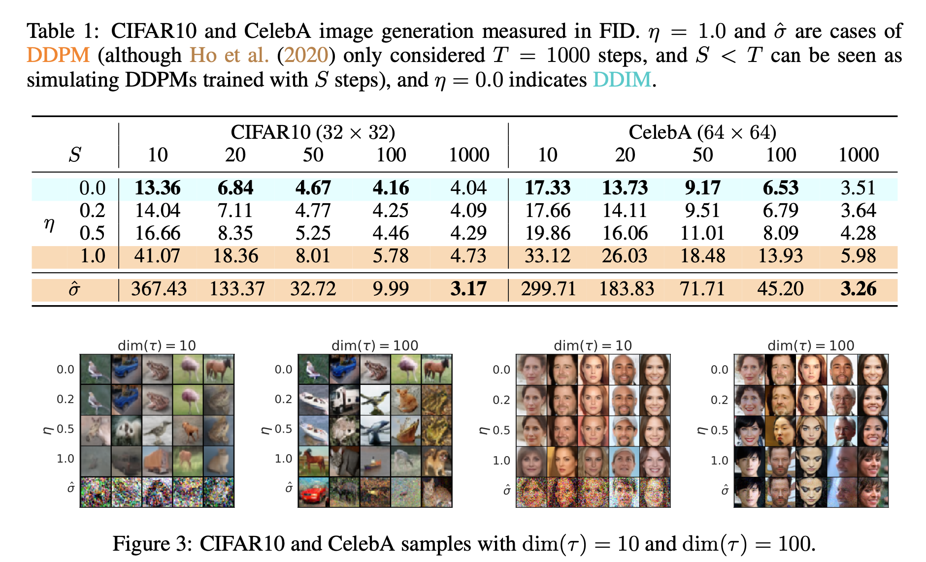
• $\hat \sigma:$Larger standard deviation
• Metric : FID
• S : timestep
• Trade-off : higher S -> better quality but more expensive computational costs.

1. Higer variance & Fewer step -> Lower quality (more noisy perturbation..)
2. DDIM achieves high sampe quality much more consistently
3. $\times$10~50 speed up compared to original DDPM

Sample Consistency

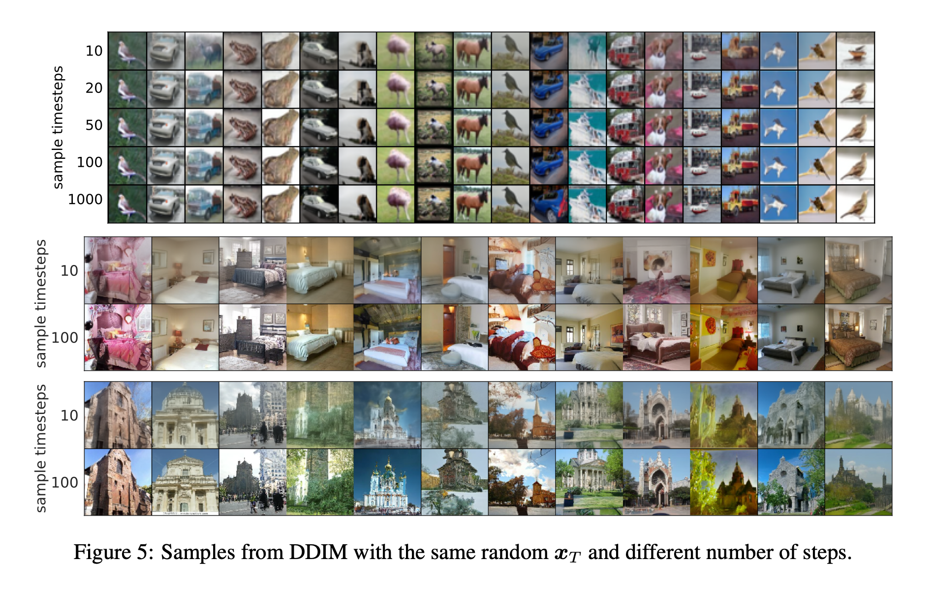
The generative process of DDIM is deterministic, so $x_0$ is depend only on the initial state $x_t$.
In order to evaluate this property (consistency), authors generated samples under different trajectories (different $\tau$).

As shown in Figure 5, although longer sample trajectories demonstrated better quality, the high-level features were not affected. This means that the high-level features are encoded by $x_T$.

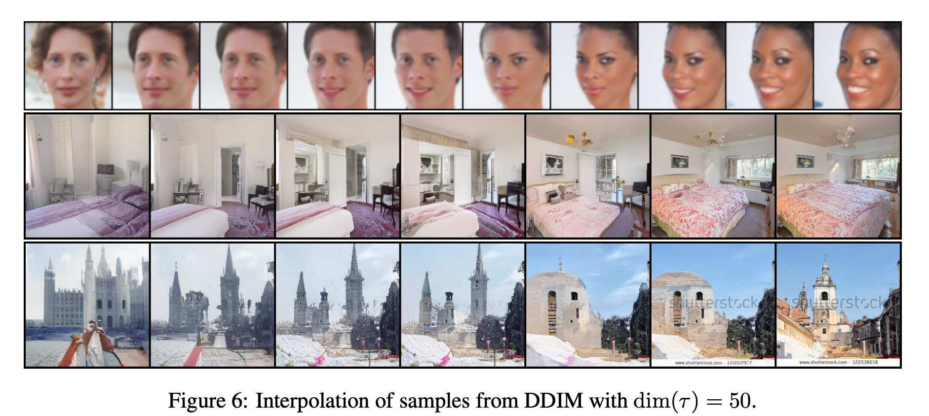
Interpolation in Deterministic Generative Processes

Interpolation in timestep $t=T$ of DDPM shows high variance. On the other hand, thanks to the consistency property, DDIM can do semantically meaningful interpolation.

Reconstruction from Latent Space

• Autoencoding with DDIM; $x_0 \rightarrow x_T \rightarrow x_0$
• DDIM successfully encoded and reconstructed, because it is the Euler integration for a particular ODE.
• DDPM cannot achieve this, due to its stochastic nature.

내 생각에 중요한점

저자가 어떻게 아이디어를 어떤 프로세스로 발전시켰는지 생각해보는게 중요해보인다. 이 흐름을 놓치면 논문이 뒤죽박죽처럼 느껴질 수 있을듯 (뇌피셜이긴하다).

1. DDPM에서 잘 작동하는 loss $L_1$ (L1 norm을 의미하는게 아님)을 보니 $q(x_t|x_0)$에만 관련있지 Markovian process가 아니더라도 성립할 수 있을 것 같다.
2. 그럼 다른 graphical model로 정의했을때도 동일한 loss를 사용하여 훈련할 수 있을듯 함 (단, 동일 schedule)
3. 그러니까 $q(x_t|x_0)$의 정의를 가장 큰 그림으로 두자. 그리고 이를 기반으로 식을 풀어나가기.
4. Non markovian으로 정의하면 바로 전 state에만 의존하지 않기도 하고 diffusion process의 continuity property를 만족하지 않아도 되니까 스텝을 조금 가져가도 괜찮을듯
5. 이후 process...