Previous post : https://velog.io/@yhyj1001/Generative-Modeling-by-Estimating-Gradients-of-the-Data-Distribution-1-A-Connection-Between-Score-Matching-Denoising-Autoencoders
github: https://github.com/yhy258/ScoreMatching_pytorch/tree/main

Motivations & Intuitions ⭐️

Motivations 📚

• The score $\nabla_x \log p_{data}(x)$ is a gradient taken in the ambient space of $x$, so it is undefined when $x$ is confined to a low dimensional manifold (manifold hypothesis).
• When the support of the data distribution is confined, the score matching objective can not be a plausible score estimator. This is because the score matching function is an expectation for the given data distribution.
• Because of the scarcity of data in low density regions, score matching may not have enough evidence to estimate score functions accurately in regions of low data density.
• When two modes of the data distribution are separated by low density regions, Langevin dynamics cannot successfully reflect the relative weights of these two modes in reasonable time, and might not result in the ground truth data distribution. This is because the score function does not depend on the relative weights of the modes.

Intuitions 🧐

• The support of Gaussian noise distributions is the whole space.
• Large Gaussian noise can fill low density regions.
• Perturbed data using various levels of noise can effectively reflect the iterative sampling method, Langevin dynamics.

Contributions ⭐️

• They perturb the data using various levels of noise.
• They propose the annealing schedule for Langevin dynamics in order to accurately reflect the relative weights of the modes.

Methods

Noise Conditional Score Networks

First of all, authors define a decreasing positive geometric sequence $\{\sigma_1, \sigma_2, \cdots, \sigma_L\}$. In addition, $q_{\sigma_i}(x) = \int p_{data}(t)\mathcal{N}(x | t, \sigma^2 I)dt$ is a sequence of noise-perturbed distributions that converge to the true data distribution.
They employ the architecture design of UNet to jointly estimate the scores of all perturbed data distribution, $s_\theta (x, \sigma) \approx \nabla_x \log q_\sigma (x)$.

Learning NCSNs via score matching

In order to perform the score matching, they use the denoising score matching. However, a sliced score matching can also train NCSNs.
As discussed in the previous post, the denoising score matching is defined as:

This equation can be defined because $q_\sigma(\tilde x|x)$ is tractable.
Then, they combine this equation for all $\sigma_i$.

where $\lambda(\sigma_i)$ is positive.
Because they observe that when the score networks are trained to optimality, $||s_\theta(x, \sigma)||_2 \approx {1\over \sigma}$, they set $\lambda(\sigma_i)$ coefficients as $\sigma^2_i$ so that the values of $\lambda(\sigma_i)l(\theta;\sigma_i)$ are soughly of the same order of magnitude.

If $\lambda(\sigma_i)= \sigma^2_i$ , $\lambda(\sigma) l (\theta;\sigma)={1\over 2}\mathbb{E}[||\sigma s_\theta(\tilde x,\sigma)+{\tilde x - x\over \sigma}||^2_2]$. In this equation, $||\sigma s_\theta(x, \sigma)||_2 \approx 1$ and ${\tilde x - x\over \sigma} \sim \mathcal{N}(0, I)$

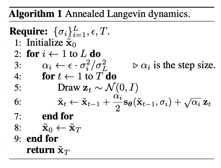
NCSN inference via annealed Langevin dynamics

• In the low density region, they employ larger step sizes.
• They can also choose $\alpha_i \approx \sigma_i^2$ in order to fix the magnitude of the "signal-to-noise" ratio in Langevin dynamics.
  Langevin sampling method with the Euler method is defined as $\tilde x_t \leftarrow \tilde x_{t-1}+{\alpha_i\over 2}s_\theta(\tilde x_{t-1}, \sigma_i) + \sqrt{\alpha_i}z_t$. According to this definition, SNR is $\alpha_i s_\theta(x, \sigma_i) \over 2\sqrt{\alpha_i}z$.
  If $\alpha_i \approx \sigma_i^2$, SNR become ${1\over 4}\mathbb{E}[||\sigma_is_\theta(x, \sigma_i)||^2_2]\approx{1\over4}$.