Depth Pro: Sharp Monocular Metric Depth in Less Than a Second 리뷰

논문 링크

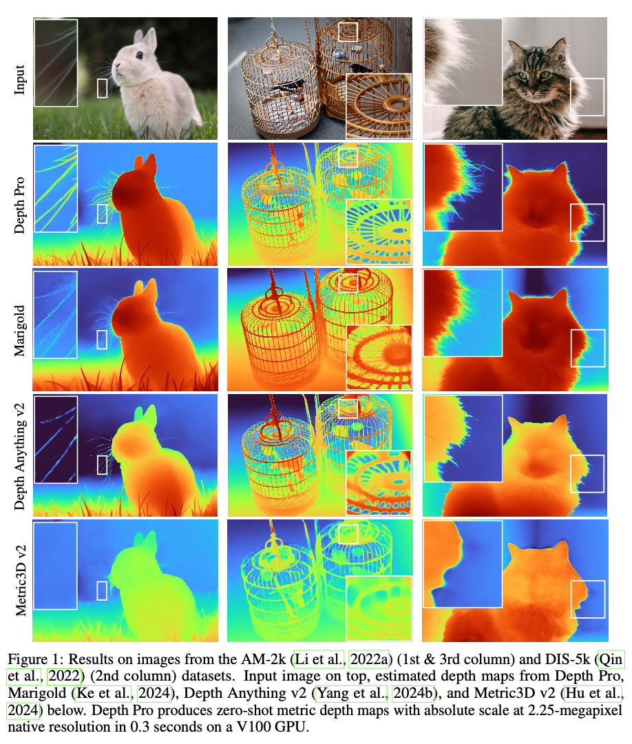
• zero-shot
• monocular
• metric

(우와)

---

Recent works

1. Zero-shot depth

이전 연구들이 사용한 methods

• 데이터셋을 엄청 많이 먹임
• scale-and-shift invariant loss (MiDaS)
• transformer-based 모델
• self-supervision
• diffusion models

이전 연구들은 모두 scale에 대해 ambiguous하다.

2. Zero-shot metric depth

이전 연구들은

• global하게 depth scale 기준을 주거나
• 특정 scene에 대한 조건을 주거나
• camera intrinsics/camera embedding를 사용하거나
• point clouds를 utilize하기 위한 별도 모델을 학습시키거나
• surface normals를 사용하거나

우리는 depth 모델에서 얻은 features에서 바로 scale을 얻어낸다.

3. Sharp occulding contours

기존 연구들은

• normals
• image patches + global context를 학습할 수 있는 추가 methods
• diffusion priors

우리는 추가적인 모듈 같은 거 안 쓰고 metric depth maps 얻으면서 더 깔끔하게 누끼 딸 수 있다.

4. 테두리 누끼 metric

• Segmentation & matting 데이터셋을 기반
• 복잡하고 다이나믹한 씬에서도 사용 가능
• GT depth를 얻을 때

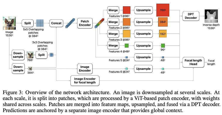
5. multi-scale ViT

우린 ViT 변형하면 다시 훈련시키기 번거로우니까 ViT 백본으로 multi-scale한 후 하나로 fuse하는 아키텍처 사용해서 global context랑 local detail 모두 사용한다.

이전 연구들 보면 pretrained ViT 모델들이 semantic segmentation이랑 object detection에 많이 사용됐다.

---

3. Method

1. 인코더 & 디코더

인코더

• ViT 인코드 그대로 사용해 pretrained ViT 백본을 갖다 씀
  • 384*384 이미지를 인풋으로 갖는 모델 사용
• 패치 크기로 원본 크기가 나눠떨어지지 않으므로 overlapping patches로 쪼갬
• Patch encoder: 여러 scale로 downsample된 이미지를 쪼개 얻은 각 패치들에 대해 scale-invariant representation을 얻을 수 있음
  • 가중치를 모든 패치에서 공유하기 때문
  • 패치마다 24*24 feature tensor를 출력
• Image encoder: 이미지를 384*384로 downsample하고 이를 Image encoder에 넣어 global context를 얻음

디코더

• DPT 모델과 유사
• 한 개의 map으로 합침

2. Sharp mono DE

Objectives

$C = f(I)$

• 각 이미지 $I$
• canonical inverse depth 이미지 $C$와 GT $\hat{C}$
  • inverse depth 사용하면 가까운 영역에 우선순위 둘 수 있어서 NVS 할 때도 좋음

$D_m = \frac{f_{px}}{wC}$

• Dense depth map $D_m$
• 시야각 (focal length) $f_{px}$
• width $w$

$\mathcal{L}_{MAE}(\hat{C}, C)=\frac{1}{N} \sum ^N_i |\hat{C}_i- C_i|$

• metric 데이터셋에서 모든 픽셀 {i}에 대해 MAE 계산
• real-world 데이터셋에서는 MAE 계산 시 각 이미지 내 상위 20% 오차를 가진 픽셀들은 discard
• non-metric 데이터셋 (intrinsics를 못 쓰거나 inconsistent scale)에 대해선 loss 계산 전 $\hat{C}$와 $C$를 정규화
  • 중간값에서 mean absolute deviation 계산해서 정규화

2. Multiscale derivative loss

• 첫 번째 & 두 번째 derivatives를 각 scale에 대해 계산함

$\mathcal{L}_{*, p, M}(C, \hat{C}) = \frac{1}{M} \sum_{j}^{M} \frac{1}{N_{j}} \sum_i^{N_j} | \nabla_* C_{i}^j - \nabla_* \hat{C}_i^j |^p$

• $M$: #scale

• $j$: inverse depth map을 scale의 2배로 blurring and downsampling해서 구함

• $\nabla_{*}$: spatial derivative operator *

  • $L$: 라플라스
  • $S$: 샤르

• $p$: norm

• MAGE (Mean Absolute Gradient Error): $\mathcal{L}_{MAGE} = \mathcal{L}_{S, 1, 6}$

• MALE (Mean Absolute Laplace Error): $\mathcal{L}_{MALE}=\mathcal{L}_{L, 1, 6}$

• MSGE (Mean Squared Gradient Error): $\mathcal{L}_{MSGE} = \mathcal{L}_{S, 2, 6}$

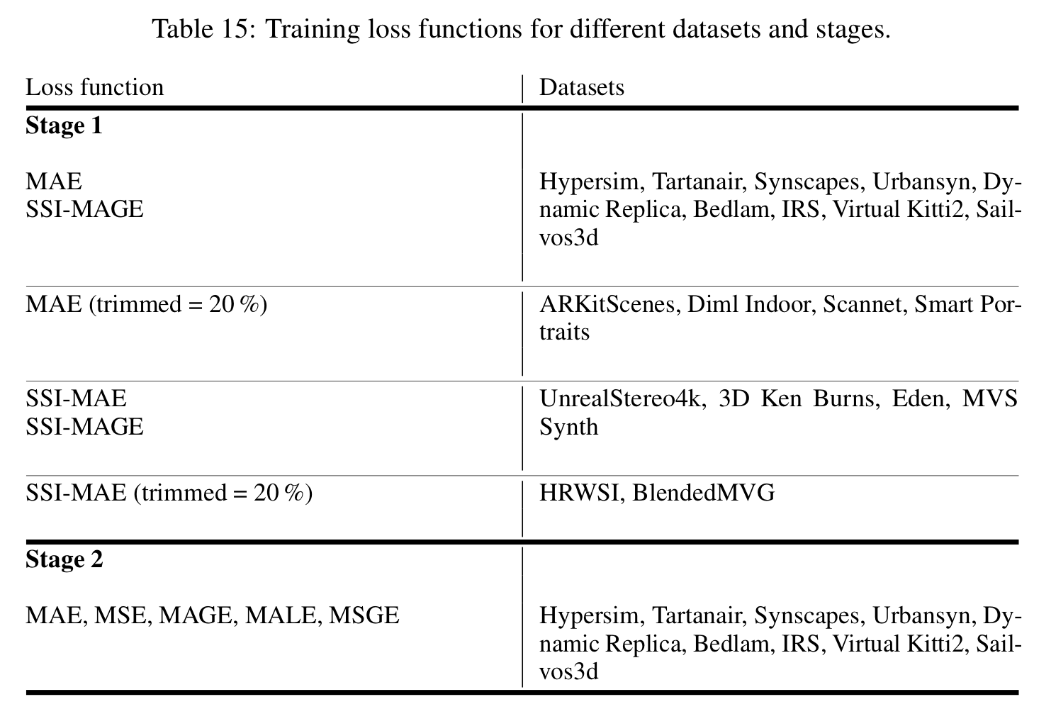
2-stage Training curriculum

보니까

• 큰 synthetic & real-world 데이터셋을 사용하면 generalize가 잘 되고
• synthetic 데이터셋과 달리 real-world 데이터셋은 depth가 완벽하지 않으며
• training course를 할수록 prediction이 샤프해지더라.

1. First stage: generalize 될 수 있도록 robust features 훈련시킴

• MAE on mixed datasets
• supervise on gradients of predictions
  • gradients에 scale-and-shift-invariant loss 쓰면 optimization이 느려져서 synthetic 데이터셋에만 적용

2. Seconds stage: 샤프한 바운더리 & 디테일

• only on synthetic data (완벽한 depth GT)
• MAE랑 gradients에 MAGE, MALE, MSGE

샤프한 바운더리 metric

• 엄청 디테일한 부분에 대해서까지 완벽한 GT depth를 얻기가 너무 어려움
• matting, saliency, segmentation에 대해서는 완벽한 GT를 찾기 쉬워서 이걸 활용
• 이 binary maps는 물체들 간의 앞뒤 배치 관계를 나타냄

$ c_d(i, j) = [ \frac{d(j)}{d(i)} > (1+ \frac{t}{100})]$

• ranking loss라는 로스식에서 영감을 얻어 이웃하는 픽셀에 대한 pairwise depth ratio 사용해 앞뒤 배치 관계를 정의
  • $c_d$ : $i$, $j$ 픽셀 간의 occluding contour
    • 배경이나 다른 물체를 가리는 (occlude하는) edges
  • $[ \cdot ]$ : Iverson bracket
    • 0이거나 1이거나
• $i$와 $j$의 depth가 $t$% 이상 차이 나면 두 픽셀 간 occluding contour
• 모든 이웃하는 픽셀에 대해 precision & recall 계산, $t$가 [5, 25]인 경우에 F1의 weighted averaging 계산함
  • $t$ 클수록 큰 weight
  • prec & recall은 scale-invariant (데이터 shape에 영향 X)
• 엣지들을 매뉴얼하게 annotate할 필요가 없고 pixelwise GT만 필요함 (synthetic 데이터셋들에서 얻기 쉬움)

Focal length estimation

• Focal length Head와 별개 인코더를 Depth estimation 학습이 끝난 후 학습시킴 (joint X)
• 메타데이터를 사용할 수 없을 경우
• L2 loss