환경설정(colab)
# 구글 드라이브 사용 권한 설정
from google.colab import drive
drive.mount('/content/gdrive/')
workspace_path = '/content/gdrive/MyDrive/경로설정/'필요 패키지 로드
import os
import cv2
import math
import torch
import random
import numpy as np
from PIL import Image
import matplotlib.pyplot as plt
import torchvision.transforms as transforms
from torchvision.transforms.functional import to_pil_image
import requests
from io import BytesIO

torch.manual_seed(17)
transforms
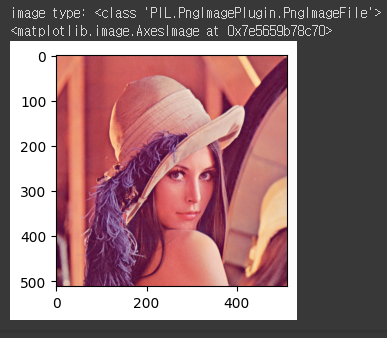
원본 이미지 확인
# img = Image.open(BytesIO(res.content))
img = Image.open('/content/gdrive/MyDrive/경로에삽입')
print('image type:', type(img))

plt.figure(figsize=(3, 3))
plt.imshow(img)
#결과:
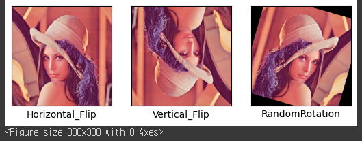
RandomHorizontal_Flip, RandomVertical_Flip, RandomRotation
Horizontal_Flip = transforms.Compose([ ##가로 방향으로 뒤집기
                                          transforms.ToTensor(),
                                          transforms.Resize((224,224)),  ##원본이미지를 224x244 사이즈로 조절
                                          transforms.RandomHorizontalFlip(p=0.5)  ##0.5확률로 어떤 이미지는 뒤집고 어떤 이미지는 뒤집지 않는다
])

Vertical_Flip = transforms.Compose([ ##세로 방향으로 뒤집기
                                          transforms.ToTensor(),
                                          transforms.Resize((224,224)),
                                          transforms.RandomVerticalFlip(p=0.5)
])

RandomRotation = transforms.Compose([ ##위치상에서
                                          transforms.ToTensor(),
                                          transforms.Resize((224,224)),
                                          transforms.RandomRotation(60)
])
## 뒤집는 이유 : 인공지능은 본대로 학습하기 때문에 어렴풋함을 인식시키기 위해 뒤집음
Horizontal_Flip_img=Horizontal_Flip(img)
Vertical_Flip_img=Vertical_Flip(img)
RandomRotation_img=RandomRotation(img)
fig = plt.figure() # rows*cols 행렬의 i번째 subplot 생성
plt.figure(figsize=(3, 3))
rows = 1
cols = 3
transform_imgs = [Horizontal_Flip_img,Vertical_Flip_img,RandomRotation_img]
xlabels = ['Horizontal_Flip','Vertical_Flip','RandomRotation']
for i,aug_img in enumerate(transform_imgs):
ax = fig.add_subplot(rows, cols, i+1)
ax.imshow(to_pil_image(aug_img))
ax.set_xlabel(xlabels[i])
ax.set_xticks([]), ax.set_yticks([])
plt.show()#결과:
ColorJitter
#밝기
bright = transforms.Compose([
                                          transforms.ToTensor(),
                                          transforms.Resize((224,224)),
                                          transforms.ColorJitter(brightness=0.5)
])

#대비
contrast = transforms.Compose([
                                          transforms.ToTensor(),
                                          transforms.Resize((224,224)),
                                          transforms.ColorJitter(contrast=0.5)
])

#채도
saturation = transforms.Compose([
                                          transforms.ToTensor(),
                                          transforms.Resize((224,224)),
                                          transforms.ColorJitter(saturation=0.5)
])

#색조
hue = transforms.Compose([
                                          transforms.ToTensor(),
                                          transforms.Resize((224,224)),
                                          transforms.ColorJitter(hue=0.5)
])

# ColorJitter : 밝기, 대비, 채도, 색조
ColorJitter=transforms.Compose([
                                          transforms.ToTensor(),
                                          transforms.Resize((224,224)),
                                          transforms.ColorJitter(brightness=0.5, contrast=0.5, saturation=0.5, hue=0.5)
])
bright_img=bright(img)
contrast_img=contrast(img)
saturation_img=saturation(img)
hue_img=hue(img)
ColorJitter_img=ColorJitter(img)
fig = plt.figure() # rows*cols 행렬의 i번째 subplot 생성
plt.figure(figsize=(3, 3))
rows = 1
cols = 5
transform_imgs = [bright_img,contrast_img,saturation_img,hue_img,ColorJitter_img]
xlabels = ['bright','contrast','saturation','hue','ColorJitter']
for i,aug_img in enumerate(transform_imgs):
ax = fig.add_subplot(rows, cols, i+1)
ax.imshow(to_pil_image(aug_img))
ax.set_xlabel(xlabels[i])
ax.set_xticks([]), ax.set_yticks([])
plt.show()#결과:
Normalize
Normalize = transforms.Compose([
                                          transforms.ToTensor(), ##자동으로 정수가 0~1로 Normalize 됨
                                          transforms.Resize((224,224)),
                                          transforms.Normalize([0.5,0.5,0.5],[0.5,0.5,0.5]) ## 평균, 편차 설정
                                          ## 정수(Numpy) : 0~255, 소수(tensor) : 0~1
])
## 데이터셋 상에 존재하는 모든 이미지의 픽셀 값 (rgb)을 불러온다
## 그리고 데이터셋 이미지 개수로 나눈다
Normalize_img=Normalize(img)
plt.figure(figsize=(3, 3))
plt.imshow(to_pil_image(Normalize_img))#결과:
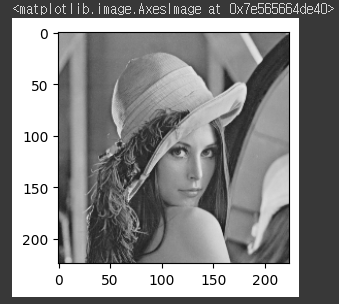
Grayscale
Grayscale = transforms.Compose([
                                          transforms.ToTensor(),
                                          transforms.Resize((224,224)),
                                          transforms.Grayscale(3) ##
])
Grayscale_img=Grayscale(img)
plt.figure(figsize=(3, 3))
plt.imshow(to_pil_image(Grayscale_img))
## RGB 이미지 -> (0~255)(0~255)(0~255) 총 3채널
## Gray 이미지 -> (0~255) 총 1채널#결과:
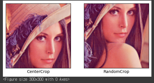
CenterCrop, RandomCrop
CenterCrop = transforms.Compose([
                                          transforms.ToTensor(),
                                          transforms.Resize((224,224)),
                                          transforms.CenterCrop(112)  ## 가운데 점을 기준으로 한 쪽 폭의 길이  ## 224x244 사이즈의 반(지름)
])

RandomCrop = transforms.Compose([
                                          transforms.ToTensor(),
                                          transforms.Resize((224,224)),
                                          transforms.RandomCrop(112)  ## 위치가 랜덤
])
CenterCrop_img=CenterCrop(img)
RandomCrop_img=RandomCrop(img)
fig = plt.figure() # rows*cols 행렬의 i번째 subplot 생성
plt.figure(figsize=(3, 3))
rows = 1
cols = 2
transform_imgs = [CenterCrop_img,RandomCrop_img]
xlabels = ['CenterCrop','RandomCrop']
for i,aug_img in enumerate(transform_imgs):
ax = fig.add_subplot(rows, cols, i+1)
ax.imshow(to_pil_image(aug_img))
ax.set_xlabel(xlabels[i])
ax.set_xticks([]), ax.set_yticks([])
plt.show()#결과:
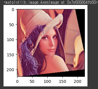
RandomAffine
RandomAffine = transforms.Compose([
                                          transforms.ToTensor(),
                                          transforms.Resize((224,224)),
                                          transforms.RandomAffine(degrees=15, translate=(0.2, 0.2),scale=(0.8, 1.2), shear=15)
])
RandomAffine_img=RandomAffine(img)
plt.figure(figsize=(3, 3))
plt.imshow(to_pil_image(RandomAffine_img))#결과:
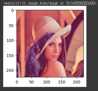
GaussianBlur
GaussianBlur = transforms.Compose([
                                          transforms.ToTensor(),
                                          transforms.Resize((224,224)),
                                          transforms.GaussianBlur((5,5), sigma=(1.0, 2.0))  ## 이미지 블러 처리
])
## 이미지가 명확하게 보이지 않을 때도 인식할 수 있게 블러처리
GaussianBlur_img=GaussianBlur(img)
plt.figure(figsize=(3, 3))
plt.imshow(to_pil_image(GaussianBlur_img))#결과:
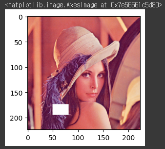
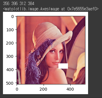
Random Erasing
RandomErasing = transforms.Compose([
                                          transforms.ToTensor(),
                                          transforms.Resize((224,224)),
                                          transforms.RandomErasing(p=1.0, scale=(0.01,0.05), ratio=(0.5,1.5), value=3)
])

#p : function 적용 확률
#scale : 전체 이미지중 erased area가 차지할 비율 (range), erased area 크기가 이미지 크기*0.01~0.05의 크기로 선택됨
#ratio : erased area의 가로,세로 해상도 비율 (range), 해상도가 0.5,1.5 중에 선택됨
#value : 3일때, 3채널을 모두 지움(v=255 for R,G,B)
RandomErasing_img=RandomErasing(img)
plt.figure(figsize=(3, 3))
plt.imshow(to_pil_image(RandomErasing_img))
## 가로 224, 세로 224인 배열 공간 안에서 랜덤한 위치(사각형)를 정하고, 그 부분을 (255, 255, 255)#결과:
코드 구현
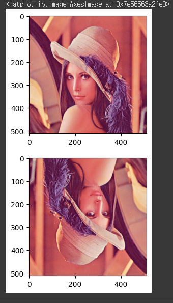
horizontal flip, vertical flip
def HorizontalFlip(img):
    img = np.fliplr(img) ## flip left right 좌우 방향으로 뒤집기
    img = Image.fromarray(np.uint8(img))
    return img

def VerticalFlip(img):
    img = np.flipud(img) ## flip up down 상하 방향으로 뒤집기
    img = Image.fromarray(np.uint8(img))
    return img
HorizontalFlip_img = HorizontalFlip(img.copy())
VerticalFlip_img = VerticalFlip(img.copy())
plt.figure(figsize=(3, 3))
plt.imshow((HorizontalFlip_img))
plt.figure(figsize=(3, 3))
plt.imshow((VerticalFlip_img))#결과:
RandomErasing
def RandomErasing(img, scale=(0.01,0.05), ratio=(0.5,1.5), value=255):
  img=img.copy()

  img = np.array(img)
  img_h, img_w, _ = img.shape
  area = img_h*img_w

  erase_area = area * torch.empty(1).uniform_(scale[0], scale[1]).item()  ## 빈 공간 정의
  aspect_ratio=torch.empty(1).uniform_(ratio[0],ratio[1]).item()

  w = int(round(math.sqrt(erase_area))) ## round : 반올림, sqrt : 제곱근
  h = int(round(w * aspect_ratio))

  patch = np.full((h,w), value) ## ((shape1, shape2), 값)의 값으로 채움  ex np.full((100,100),0) -> 0으로 채워진 (100, 100) 생성  ## 1채널
  patch=np.repeat(patch[:,:,np.newaxis], 3, -1)
  h_range,w_range=img_h-h,img_w-w
  h = random.randrange(0, h_range) ## 해당범위 랜덤
  w = random.randrange(0, w_range)

  print(h,h+patch.shape[0],w,w+patch.shape[1])
  img[h:h+patch.shape[0], w:w+patch.shape[1],:]=patch  ## 영역을 지정하고 patch의 값을 대입

  # np.putmask(img, patch, value)

  img = Image.fromarray(np.uint8(img))

  return img
RandomErasing_img = RandomErasing(img.copy())
plt.figure(figsize=(3, 3))
plt.imshow(RandomErasing_img)#결과:
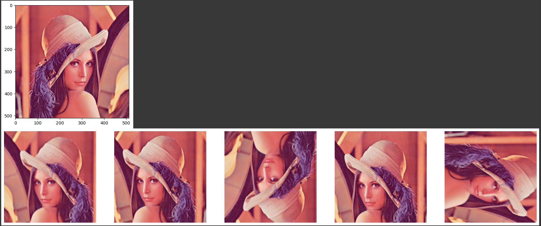
Albumentations
- Albumentations 설치
!pip install -U albumentationsimport albumentations as A
albumentations_transform_oneof = A.Compose([
A.Resize(256, 256),
A.RandomCrop(224, 224),
A.OneOf([
A.HorizontalFlip(p=1),
A.ShiftScaleRotate(p=1),
A.RandomRotate90(p=1),
A.HueSaturationValue(p=1),
A.Cutout(p=1, num_holes=8, max_h_size=24, max_w_size=24)
], p=1),
A.OneOf([
A.MotionBlur(p=1),
A.OpticalDistortion(p=1),
A.GaussNoise(p=1),
], p=1),
])
albumentations_image = albumentations_transform_oneof(image=np.array(img.copy()))
albumentations_image = Image.fromarray(albumentations_image['image'])
plt.imshow(img)
plt.show()
num_samples = 5
fig, ax = plt.subplots(1, num_samples, figsize=(25, 5))
for i in range(num_samples):
albumentations_image = albumentations_transform_oneof(image=np.array(img.copy()))['image']
ax[i].imshow(albumentations_image)
ax[i].axis('off')
plt.show()#결과:

공부 기록