진득히 공부할 시간이 없네...
학습시간 09:00~02:00(당일17H/누적751H)
◆ 학습내용
U-Net으로 축구 경기 객체 분할하기
어제(1번~6번)에 이어 7번 시작!
7. 데이터셋 클래스 생성
def train_transform():
    return A.Compose([
        A.Resize(256, 256),
        A.HorizontalFlip(p=0.5),
        A.RandomBrightnessContrast(p=0.2),
        A.Affine(translate_percent=0.1, scale=(0.9, 1.1), rotate=(-15, 15), p=0.5),
        A.Normalize(),
        ToTensorV2()
    ])

def test_transform():
    return A.Compose([
        A.Resize(256, 256),
        A.Normalize(),
        ToTensorV2()
    ])
클래스 생성 전에 데이터 증강에 사용할 함수 2개를 만들었다.
원래 변수로 저장했는데, 이번엔 함수로 저장해서 사용해 보려고 한다. 함수로 만들면 함수명에 색상이 부여되어서 가독성이 조금 좋아지는 것 같음.
라이브러리는 v2대신 탐지 때 알아낸 Albumentations를 사용했다. bbox가 있으면 또 뒤에 bbox~.format='' 을 넣어줘야 하는데, 이번엔 필요 없는 것 같다.
여기서 조금 특이한 것은 Affine 증강인데, 파라미터에 넣은 값들이 p확률 만큼 랜덤적용된다고 한다.
class FootballDataset(Dataset):
    def __init__(self, image_dir, mask_dir, image_files, transform=None):
        self.image_dir = image_dir
        self.mask_dir = mask_dir
        self.image_files = image_files
        self.transform = transform

    def __len__(self):
        return len(self.image_files)
FootballDataset 도입부를 만들었다.
- 원본 이미지 폴더 경로
- 어제 만든 마스크 폴더 경로
- 훈련&평가 나눌 기준
- 데이터증강 나눌 기준
이렇게 파라미터로 넣었다.
    def __getitem__(self, idx):
        filename = self.image_files[idx]
        img_path = os.path.join(self.image_dir, filename)
        mask_path = os.path.join(self.mask_dir, filename)

        image = np.array(Image.open(img_path).convert("RGB"))
        mask = np.array(Image.open(mask_path))

        augmented = self.transform(image=image, mask=mask)
        image = augmented['image']
        mask = augmented['mask']
다음은 getitem 부분이다.
파일명으로 이미지&마스크를 매핑하고, 데이터 증강을 위해 다시 둘로 나눈다.
이미지는 RGB 형태로 바꿔준다.
train_files, test_files = train_test_split(image_dir, test_size=0.2, random_state=42)

train_dataset = FootballDataset(
    image_dir=DIR['data'] + '/FootballSegmentation/images',
    mask_dir=DIR['data'] + '/FootballSegmentation/masks',
    image_files=train_files,
    transform=train_transform()
)

test_dataset = FootballDataset(
    image_dir=DIR['data'] + '/FootballSegmentation/images',
    mask_dir=DIR['data'] + '/FootballSegmentation/masks',
    image_files=test_files,
    transform=test_transform()
)
데이터를 train, test로 나눴다.
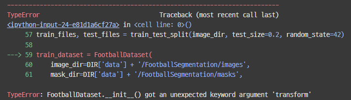
??? 에러가 떴다.
헉 ㅋ init 에 transform을 안 넣었다.
class FootballDataset(Dataset):
    def __init__(self, image_dir, mask_dir, image_files, transform):
        self.image_dir = image_dir
        self.mask_dir = mask_dir
        self.image_files = image_files
        self.transform = transform
후다닥 넣고,
train_loader = DataLoader(dataset=train_dataset, batch_size=8, shuffle=True)
test_loader = DataLoader(dataset=test_dataset, batch_size=8, shuffle=True)
로더도 만들어 주고,
for image, mask in train_loader:
    print(image.shape)
    print(mask.shape)
    break
잘 만들어졌는지 테스트해 보자.
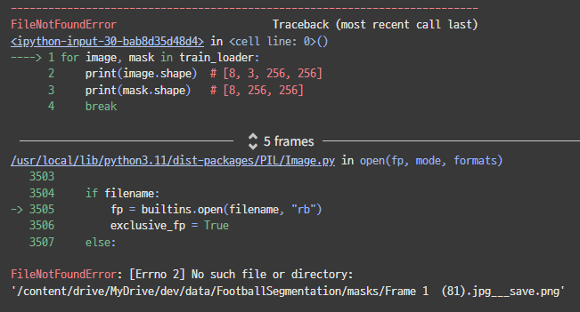
또 에러네.
이상하다...?? Frame 1 (81).jpg___save.png 파일이 없다고 한다.
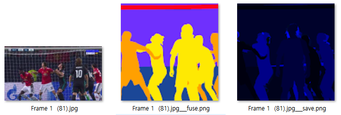
여기서 세 번째 파일을 찾고 있는 것 같다.
이거는 필요 없는 파일아닌가,,,
하.. ㅠㅠ 쉽게 되는 게 하나도 없네.
다행이도 첫 번째 파일이 jpg이다. 이 확장자만 찾도록 바꾸면 될 것 같다.
train_images = [f for f in os.listdir(image_dir) if f.endswith('.jpg')]
train_files, test_files = train_test_split(train_images, test_size=0.2, random_state=42)
데이터를 나눌 때 이미지 폴더에 jpg로 끝나는 100장만 찾도록 했다.
for image, mask in train_loader:
    print(f'Image: {image.shape}')
    print(f'Mask: {mask.shape}')
    break
다시 확인해 보자.
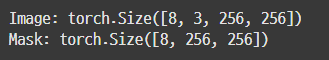
휴 이제 나온다.
8. Attention U-Net에 관하여
이번 미션에서는 U-Net을 사용하라고 했다.
하지만, 나는 오토인코더 미션 때 논문을 보면서 U-Net을 구현해본 적이 있기 때문에 이번엔 다른 걸 해보려 한다.
Attention U-Net 모델을 만들어 보자.
일단 공부를 좀 해보자.
가볍게 논문 슥 훑어보자.
AG 라는 게 유넷 모델 성능을 향상시켰다고 한다.
첫 줄에 있듯, AG는 Attention Gate의 약자다.
RNN에 Forget Gate를 접목한 것과 비슷한 느낌인가??
일단 조금 더 읽어 보자.
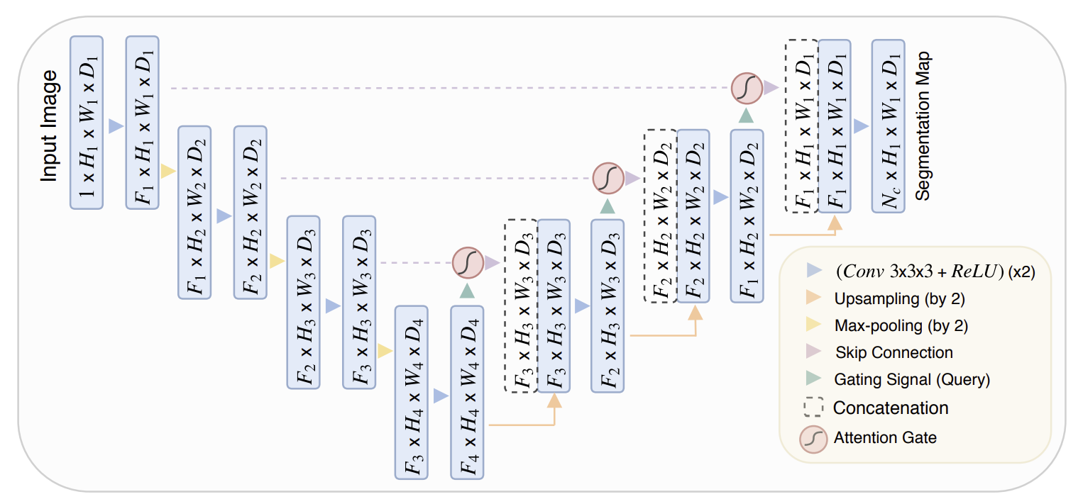
조금 더 내려보니 모델 구조 이미지가 있다. 아따 보기 어렵게도 만들어 놨네.
이미지만 놓고 보자면, 기본 구조는 U자 형태를 유지하고 있다.
Skip Connection도 그대로 있고, 디코더 부분에 더블 채널도 그대로 있다.
추가된 건 Attention Gate와 Gating Signal이다.
Gating Signal → Attention Gate → Gating Signal 이렇게가 한 세트인 것 같다.
어텐션 기능을 지닌 스킵 커넥션인지, 아니면 어텐션을 먼저 하고 커넥션을 하는 것인지는 조금 더 읽어봐할 거 같다.
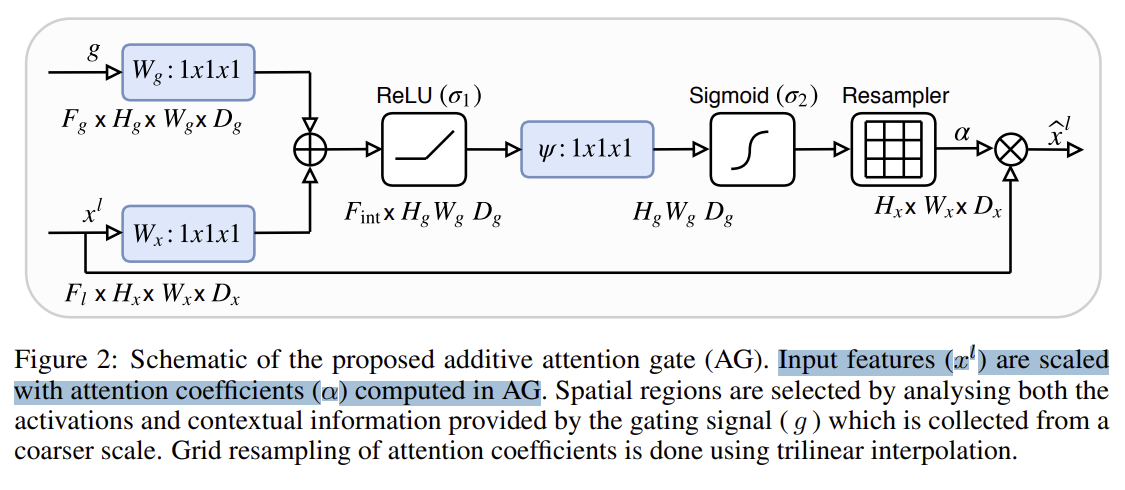
Attention Gate의 구조도 나와있다.
음,,, 수학적인 개념은 잘 모르겠지만, 어쨌든 기존 인코더에서 들어온 값(x^l)이 두 개로 나뉜다.
하나는 어텐션 게이트에 들어가고, 다른 하나는 디코더에 들어가는 것 같다.
g는 gating signal이다. 디코딩 시 바로 전단계의 아웃풋인 것 같다. 이게 인코더에서 온 값과 합쳐진 후 Attention Gate에 들어간다.
AG는 렐루와 시그모이드를 거쳐서 리샘플러라는 곳을 통과한다.
그렇군. 그러니까 쉽게 말해, 똑같은 Skip connection 이긴 하지만, 인코더 정보를 있는 그대로 concatenate 하지 않겠다는 것이다.
인코더 정보를 선별해서 합치는 것. 그게 Attention U-Net의 핵심인 것 같다.
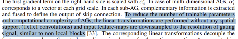
Attention gate에서는 파라미터를 줄이고 해상도를 맞추기 위해 1x1 conv를 사용한다고 한다.
어렵군,, 아무래도 모델 구현을 위한 클래스가 3개~4개 정도 필요할 것 같은 느낌이다.
9. 모델 생성
이제 본격적으로 모델을 만들어 보자.
class ConvBlock(nn.Module):
    def __init__(self, in_c, out_c):
        super().__init__()
        self.block = nn.Sequential(
            nn.Conv2d(in_c, out_c, 3, 1, 1),
            nn.BatchNorm2d(out_c),
            nn.ReLU(inplace=True),
            nn.Conv2d(out_c, out_c, 3, 1, 1),
            nn.BatchNorm2d(out_c),
            nn.ReLU(inplace=True),
        )

    def forward(self, x):
        return self.block(x)
일단 모델 안에 들어갈 더블 레이어 클래스를 만들었다.
이것도 계속 보다보니까 이제 익숙하네.
class AttentionUNet(nn.Module):
    def __init__(self):
        super().__init__()
        # Encoder
        self.encoder1 = ConvBlock(3, 64)
        self.pool1 = nn.MaxPool2d(2, 2)
        self.encoder2 = ConvBlock(64, 128)
        self.pool2 = nn.MaxPool2d(2, 2)
        self.encoder3 = ConvBlock(128, 256)
        self.pool3 = nn.MaxPool2d(2, 2)
        self.encoder4 = ConvBlock(256, 512)
        self.pool4 = nn.MaxPool2d(2, 2)

        # bottleneck
        self.bottleneck = ConvBlock(512, 1024)

    def forward(self, x):
        # Encoder
        down1 = self.encoder1(x)
        down2 = self.encoder2(self.pool1(down1))
        down3 = self.encoder3(self.pool2(down2))
        down4 = self.encoder4(self.pool3(down3))

        # Bottleneck
        bottleneck = self.bottleneck(self.pool4(down4))
메인 모델 내부에 인코더를 만들었다.
이제 디코더와 어텐션 게이트를 추가해야 하는데,,, 이건 어떻게 만들어야 하지??
잘 설명해준 블로그를 찾았다.
1x1 conv에 통과시켜 인코더 디코더 차원을 맞추어 주는 작업이 필요하다.
ReLU와 Sigmoid에 통과시켜 0~1 사이의 어텐션 계수를 만들어야 한다.
여기서 소프트맥스가 아닌 시그모이드를 사용한 이유는 소프트맥스의 결과값이 상대적으로 0에 가까운 값이 더 많아 sparse해질 수 있기 때문이다.
이 계수가 1에 가까울 수록 더 집중해서 봐야할 영역이라는 뜻이다.
그러니까 크게 보면 필요한 작업은 3가지다.
(1)
Decoder Feature (g) → Conv1x1
Encoder Feature (x) → Conv1x1
이 두 개를 더하는 부분.
(2)
여기에
ReLU → Conv1x1 → Sigmoid → α
이렇게 통과시켜서 α 값을 구하는 부분.
(3)
이렇게 나온 α값에 처음 추출한 인코더 x값을 다시 곱해주는 부분
이렇게 하면 어텐션 게이트를 통과한 인코더 블럭 값이 나오는 것이다.
오케이 이해했다.
class AttentionGate(nn.Module):
    def __init__(self, g, x, gate_channel):
        super().__init__()

        # Decoder 채널 변환
        self.g_transform = nn.Sequential(
            nn.Conv2d(g, gate_channel, 1, 1, 0),
            nn.BatchNorm2d(gate_channel)
        )

        # Encoder 채널 변환
        self.x_transform = nn.Sequential(
            nn.Conv2d(x, gate_channel, 1, 1, 0),
            nn.BatchNorm2d(gate_channel)
        )

        # Attention 계수 생성 레이어
        self.sigmoid_layer = nn.Sequential(
            nn.Conv2d(gate_channel, 1, 1, 1, 0),
            nn.BatchNorm2d(1),
            nn.Sigmoid()
        )

        self.relu = nn.ReLU(inplace=True)
init 부터 만들었다.
Decoder(g)와 Encoder(x)의 채널을 맞추기 위해 둘을 입력으로 받아서 gate_channel로 통일해준다.
전부 1x1 conv에 통과 후 시그모이드로 어텐션 계수를 뽑아준다.
    def forward(self, g, x):
        g_transformed = self.g_transform(g)
        x_transformed = self.x_transform(x)

        a = self.relu(g_transformed + x_transformed)

        a = self.sigmoid_layer(a)

        attention_feature = x * a

        return attention_feature
만든 그대로 순전파한다.
디코더(g)와 인코더(x) 채널을 통합하고,
두 개를 더해서 렐루와 시그모이드를 통과시킨다.
그렇게 나온 attention 계수(a)를
인코더(x) 정보와 곱해준다.
논문으로 볼 땐 엄청 어려웠는데 코드로 보니까 그나마 괜찮은 것 같다.
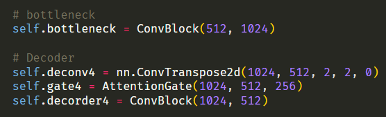
# bottleneck
self.bottleneck = ConvBlock(512, 1024)
# Decoder
self.deconv4 = nn.ConvTranspose2d(1024, 512, 2, 2, 0)
self.gate4 = AttentionGate(1024, 512, 256)
self.decorder4 = ConvBlock(1024, 512)
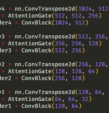
self.deconv3 = nn.ConvTranspose2d(512, 256, 2, 2, 0)
self.gate3 = AttentionGate(512, 256, 128)
self.decorder3 = ConvBlock(512, 256)
self.deconv2 = nn.ConvTranspose2d(256, 128, 2, 2, 0)
self.gate2 = AttentionGate(256, 128, 64)
self.decorder2 = ConvBlock(256, 128)
self.deconv1 = nn.ConvTranspose2d(128, 64, 2, 2, 0)
self.gate1 = AttentionGate(128, 64, 32)
self.decorder1 = ConvBlock(128, 64)
# Output
self.classifier = nn.Conv2d(64, 12, 1, 1, 0) 이제 방금 만든 AttentionGate 클래스를 유넷 모델 init 디코더 부분에 넣어준다.
Gate에서 인코더&디코더 채널 통합은 256부터 2배씩 감소하는 것으로 했다.
마지막은 아웃 채널은 11개 클래스 + 배경이니까 12로 했다.
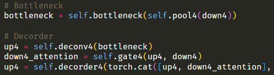
    def forward(self, x):
        # Encoder
        down1 = self.encoder1(x)
        down2 = self.encoder2(self.pool1(down1))
        down3 = self.encoder3(self.pool2(down2))
        down4 = self.encoder4(self.pool3(down3))

        # Bottleneck
        bottleneck = self.bottleneck(self.pool4(down4))

        # Decorder
        up4 = self.deconv4(bottleneck)
        down4_attention = self.gate4(up4, down4)
        up4 = self.decorder4(torch.cat([up4, down4_attention], dim=1))

        up3 = self.deconv3(up4)
        enc3_gate = self.gate3(up3, down3)
        up3 = self.decorder3(torch.cat([up3, enc3_gate], dim=1))

        up2 = self.deconv2(up3)
        enc2_gate = self.gate2(up2, down2)
        up2 = self.decorder2(torch.cat([up2, enc2_gate], dim=1))

        up1 = self.deconv1(up2)
        enc1_gate = self.gate1(up1, down1)
        up1 = self.decorder1(torch.cat([up1, enc1_gate], dim=1))

        # Output
        out = self.classifier(up1)
        return out
유넷 모델 순전파 부분을 만들었다.
전반적으로 기존 유넷모델과 구조가 똑같다.
디코더 부분에 gate가 있다는 것만 다른데, 그냥 입력을 받아서 어텐션 게이트에 넘긴 후 나온 a * x 출력값을 이전 레이어 출력값과 concatenate 해주는 게 끝이다.
device = torch.device('cuda' if torch.cuda.is_available() else 'cpu')
AttentionUNet = AttentionUNet().to(device)

summary(AttentionUNet, (8, 3, 256, 256))
이제 모델 전원을 켤 시간이다.
어떻게 생겼나 보자!
과연 잘 만들어졌을까!?
두근두근....
^^....
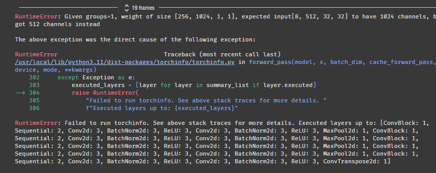
에러가 떴다. 역시 한번에 될 리가 없지!
expected input[8, 512, 32, 32] to have 1024 channels, but got 512 channels instead
1024 채널이 와야 하는데 512 채널이 와서 터졌다고 한다.
아무래도 이 부분이 문제가 된 것 같다.
코드가 길어지니까 헷갈린다... 순전파랑 비교하면서 봐야겠다.
에러에서 1024 채널을 입력으로 받아야하는데, 512 채널을 입력으로 받아서 모델이 터졌다고 했다.
1024 채널을 입력으로 받는 층은 deconv4, gate4, decorder4 셋 중 하나다.
에러에서 512 채널을 입력으로 받아서 모델이 터졌다고 했다.
근데 512 채널이 출력으로 나오는 층은 deconv4, decorder4 둘 중 하나다.
decorder4 출력값은 어차피 다음 레이어로 넘어가니까 상관없을 것이다.
그럼 deconv4 출력값이 문제라는 뜻인데,,,
nn.ConvTranspose2d(1024, 512
여기서 나오는 512 채널을
AttentionGate(1024, 512
여기에서 못받고 있는 것 같다.
그럼 ConvTranspose2d 출력을 1024로 바꾸거나, AttentionGate 첫 입력을 512로 바꾸면 될 것 같다.
AttentionGate의 첫 입력을 ConvTranspose2d 출력값과 일치시켰다.
summary(AttentionUNet, (8, 3, 256, 256))다시 확인해 보자!
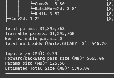
나온다!!
파라미터가 약 3,100만 개다. 엄청나네;;
이거 학습이 몇 시간이나 걸릴지 가늠이 안 된다.
10. 모델 학습
def train(model, dataloader, epochs):
    criterion = nn.CrossEntropyLoss()
    optimizer = optim.Adam(model.parameters(), lr=0.0001)
    scheduler = ReduceLROnPlateau(optimizer, factor=0.75, patience=2)

    for epoch in range(epochs):
        model.train()
        total_loss = 0

        for images, masks in tqdm(dataloader):
            images, masks = images.to(device), masks.to(device)

            outputs = model(images)
            loss = criterion(outputs, masks)

            optimizer.zero_grad()
            loss.backward()
            optimizer.step()

            total_loss += loss.item()

        print(f"[{epoch+1}/{epochs}] Loss: {total_loss/len(dataloader):.4f}")
        scheduler.step(total_loss/len(dataloader))
학습용 함수를 만들었다.
이렇게 간단해도 괜찮나 싶을 정도로 뭐가 없다.
처음엔 이 코드도 이해가 안 갔는데, 그새 많이 성장한 것 같다.
데이터가 별로 없어서 에폭을 많이 돌려야할 것 같다.
스케줄러를 넣어서 2에폭 동안 로스가 줄어들지 않으면 learning rate이 기존의 75%로 감소하도록 했다.
일단 잘 돌아가나 확인 해보자.
train(AttentionUNet, train_loader, 5)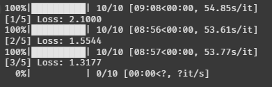
잘 돌아간다. 에폭도 잘 줄어드는 것처럼 보인다.
얼마나 돌리지? 한 200에폭 돌려볼까?
train(AttentionUNet, train_loader, 200)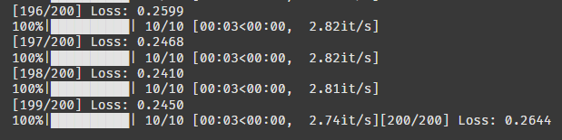
객체 탐지에 비해 학습이 엄청 금방 끝났다.
200 에폭 돌렸는데 로스가 0.26 나왔다.
100 에폭 쯤부터 내려가지 않는 걸 보니까 뭔가 최적화가 안 된 듯하다.
11. 모델 시각화 & 평가
def visualize_prediction(model, dataset, image_index):
    model.eval()
    image, mask = dataset[image_index]
    image_input = image.unsqueeze(0).to(device)

    with torch.no_grad():
        output = model(image_input)
        pred = torch.argmax(output.squeeze(), dim=0).cpu().numpy()

        unique_gt = torch.unique(mask).cpu().numpy()
    unique_pred = np.unique(pred)
    all_classes = np.union1d(unique_gt, unique_pred)
    min_class, max_class = int(all_classes.min()), int(all_classes.max())

    fig, ax = plt.subplots(1, 3, figsize=(15, 5))
    ax[0].imshow(image.permute(1, 2, 0).cpu())
    ax[0].set_title("Input Image")

    ax[1].imshow(mask.cpu(), cmap='tab20', vmin=min_class, vmax=max_class)
    ax[1].set_title(f"Ground Truth ({len(unique_gt)} classes)")

    ax[2].imshow(pred, cmap='tab20', vmin=min_class, vmax=max_class)
    ax[2].set_title(f"Prediction ({len(unique_pred)} classes)")

    plt.show()
시간이 없어서 급조로 만들었다... ㅠㅠ
image_index = 5

visualize_prediction(AttentionUNet, test_dataset, image_index=image_index)
5번 사진만 확인해 보자.
tab20 이라는 컬러맵을 사용하면 모든 클래스가 구분되어서 나오는 것 같다. 완전 꿀팁!
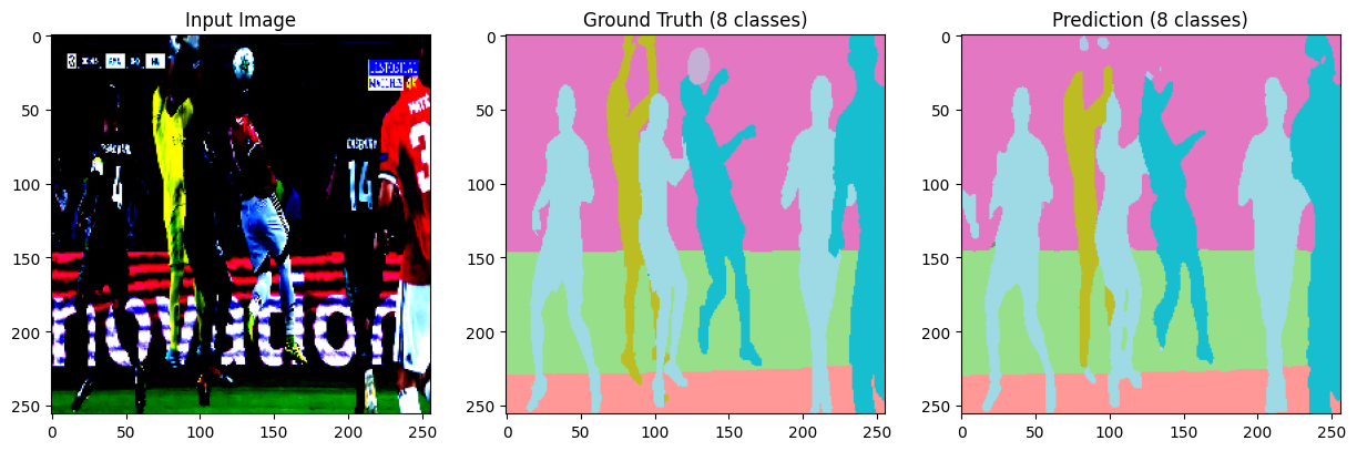
음... 어느정도 식별은 한 것 같은데, 축구공은 미처 찾지 못한 것 같다.
하긴 로스가 높으니 성능이 안 좋겠다고 생각하긴 했다.
def evaluate_prediction_named(model, dataset, image_index):
    idx_to_name = {
    v: cat['name']
    for cat in helper.categories
    for k, v in helper.category_map.items()
    if k == cat['id']
    }

    model.eval()
    image, gt_mask = dataset[image_index]
    image_input = image.unsqueeze(0).to(device)

    with torch.no_grad():
        output = model(image_input)
        pred_mask = torch.argmax(output.squeeze(), dim=0).cpu()


    classes = torch.unique(torch.cat([gt_mask, pred_mask])).tolist()

    print(f"\n▶ Dice Score by Class (Image Index: {image_index}) ◀")
    for cls in sorted(classes):
        gt_cls = (gt_mask == cls).int().flatten()
        pred_cls = (pred_mask == cls).int().flatten()

        intersection = (gt_cls & pred_cls).sum().item()
        total = gt_cls.sum().item() + pred_cls.sum().item()

        dice = (2. * intersection) / total if total > 0 else 1.0
        name = idx_to_name.get(cls, f"Class {cls}")
        print(f" - {dice:.2f}: {name}")
평가지표로는 DICE SCORE를 사용했다.
DICE는 분할 테스크에서 많이 사용하는 지표라고 한다.
특이하게 매트릭으로도 사용할 수 있고 손실함수로도 사용할 수 있는 것 같다.
image_index = 5

evaluate_prediction_named(AttentionUNet, test_dataset, image_index=image_index)
아까 5번 사진 수치를 보자!
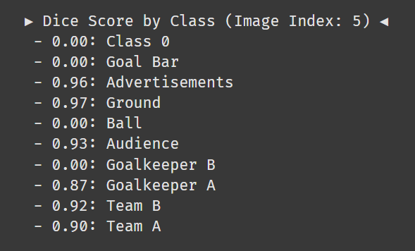
음 확실히 축구공을 아예 못찾았다.
찾은 클래스는 배경과 광고간판 제외하면 87점~93점이다. 썩 좋진 않지만 썩 나쁘지도 않다.
모델 성능 개선하고 더 공부하고 싶은데 시간이 없네.
모르겠다. 이번 미션은 여기서 끝!
기회가 되면 또 보자 나의 유넷!!!