
1. 개발환경과 데이터셋
💻 개발환경: Google Colab
✅ 사용 데이터셋
(MBTI) Myers-Briggs Personality Type Dataset
[Link] https://www.kaggle.com/datasets/datasnaek/mbti-type
mbti_1.csv
MBTI Personality Types 500 Dataset
[Link] https://www.kaggle.com/datasets/zeyadkhalid/mbti-personality-types-500-dataset
MBTI 500.csv
kaggle에 있는 2개의 MBTI 데이터셋을 사용했습니다.
type, posts 2개의 열을 가진 데이터로, type은 mbti 종류이며 posts는 해당 mbti가 작성한 텍스트 데이터입니다.
❤️저는 colab을 아주 애용하기 때문에 이번 프로젝트도 colab을 사용하여 개발을 진행하였습니다.❤️
2. 데이터 전처리
from google.colab import drive
drive.mount('/content/drive')

import pandas as pd
import numpy as np
import warnings
warnings.filterwarnings('ignore')

import seaborn as sns
import matplotlib.pyplot as plt

#데이터셋 로드
data = pd.read_csv('/content/drive/MyDrive/spp_project/mbti_concat.csv')
위 코드에서 로드한 데이터셋은 사전에 2개의 데이터셋을 합친 csv 파일입니다.
data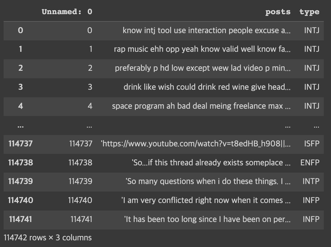
데이터셋을 합치면서 생성된 'Unnamed: 0' 컬럼이 보입니다. concat()을 진행하는 과정에서 index가 하나 더 생긴 것 같습니다. 불필요하기 때문에 해당 열 전체를 삭제해줍니다.
# 불필요한 열 제거
data = data.drop(['Unnamed: 0'], axis=1)
data
해당 열이 삭제된 것을 확인되었으니 본격적인 전처리를 시작하겠습니다.
영어에는 '축약형'이라는 것이 존재하기 때문에 이러한 텍스트를 정제하는 과정을 거쳐야 합니다. 아래의 링크를 참고하여 코드를 작성하였습니다.
https://stackoverflow.com/questions/19790188/expanding-english-language-contractions-in-python
# 전처리 함수에서 사용할 contractions 생성
contractions = {"'cause": 'because',
 "I'd": 'I would',
 "I'd've": 'I would have',
 "I'll": 'I will',
 "I'll've": 'I will have',
 "I'm": 'I am',
 "I've": 'I have',
 "ain't": 'is not',
 "aren't": 'are not',
 "can't": 'cannot',
 "could've": 'could have',
 "couldn't": 'could not',
 "didn't": 'did not',
 "doesn't": 'does not',
 "don't": 'do not',
 "hadn't": 'had not',
 "hasn't": 'has not',
 "haven't": 'have not',
 "he'd": 'he would',
 "he'll": 'he will',
 "he's": 'he is',
 "here's": 'here is',
 "how'd": 'how did',
 "how'd'y": 'how do you',
 "how'll": 'how will',
 "how's": 'how is',
 "i'd": 'i would',
 "i'd've": 'i would have',
 "i'll": 'i will',
 "i'll've": 'i will have',
 "i'm": 'i am',
 "i've": 'i have',
 "isn't": 'is not',
 "it'd": 'it would',
 "it'd've": 'it would have',
 "it'll": 'it will',
 "it'll've": 'it will have',
 "it's": 'it is',
 "let's": 'let us',
 "ma'am": 'madam',
 "mayn't": 'may not',
 "might've": 'might have',
 "mightn't": 'might not',
 "mightn't've": 'might not have',
 "must've": 'must have',
 "mustn't": 'must not',
 "mustn't've": 'must not have',
 "needn't": 'need not',
 "needn't've": 'need not have',
 "o'clock": 'of the clock',
 "oughtn't": 'ought not',
 "oughtn't've": 'ought not have',
 "sha'n't": 'shall not',
 "shan't": 'shall not',
 "shan't've": 'shall not have',
 "she'd": 'she would',
 "she'd've": 'she would have',
 "she'll": 'she will',
 "she'll've": 'she will have',
 "she's": 'she is',
 "should've": 'should have',
 "shouldn't": 'should not',
 "shouldn't've": 'should not have',
 "so's": 'so as',
 "so've": 'so have',
 "that'd": 'that would',
 "that'd've": 'that would have',
 "that's": 'that is',
 "there'd": 'there would',
 "there'd've": 'there would have',
 "there's": 'there is',
 "they'd": 'they would',
 "they'd've": 'they would have',
 "they'll": 'they will',
 "they'll've": 'they will have',
 "they're": 'they are',
 "they've": 'they have',
 "this's": 'this is',
 "to've": 'to have',
 "wasn't": 'was not',
 "we'd": 'we would',
 "we'd've": 'we would have',
 "we'll": 'we will',
 "we'll've": 'we will have',
 "we're": 'we are',
 "we've": 'we have',
 "weren't": 'were not',
 "what'll": 'what will',
 "what'll've": 'what will have',
 "what're": 'what are',
 "what's": 'what is',
 "what've": 'what have',
 "when's": 'when is',
 "when've": 'when have',
 "where'd": 'where did',
 "where's": 'where is',
 "where've": 'where have',
 "who'll": 'who will',
 "who'll've": 'who will have',
 "who's": 'who is',
 "who've": 'who have',
 "why's": 'why is',
 "why've": 'why have',
 "will've": 'will have',
 "won't": 'will not',
 "won't've": 'will not have',
 "would've": 'would have',
 "wouldn't": 'would not',
 "wouldn't've": 'would not have',
 "y'all": 'you all',
 "y'all'd": 'you all would',
 "y'all'd've": 'you all would have',
 "y'all're": 'you all are',
 "y'all've": 'you all have',
 "you'd": 'you would',
 "you'd've": 'you would have',
 "you'll": 'you will',
 "you'll've": 'you will have',
 "you're": 'you are',
 "you've": 'you have'}
데이터셋에서 유의미한 단어 토큰만을 선별하기 위해서 큰 의미가 없는 단어 토큰을 제거하는 과정이 필요합니다. 예를 들어, 'I', 'my', 'me', 조사, 접미사 등과 같은 단어들은 문장에 빈번하게 등장하지만 의미 분석을 하는데는 많은 기여를 하지 않는 경우가 많습니다. 이러한 단어들을 불용어(stopword)라고 하며, nltk에는 불용어들을 패키지 내에서 미리 정의하고 있습니다.
nltk의 불용어를 사용하기위한 모듈을 import해야 하는데, 만약 데이터가 없다는 에러가 발생하면 nltk.download라는 커맨드를 통해서 다운로드가 가능합니다.
import nltk
nltk.download('stopwords')
from nltk.corpus import stopwords

# NLTK의 불용어
stop_words = set(stopwords.words('english'))
print('불용어 개수 :', len(stop_words))
print(stop_words)
stopwords.words("english")는 nltk가 정의한 영어 불용어 리스트를 반환해줍니다. 위의 코드로 불용어의 개수와 불용어를 출력해서 확인할 수 있습니다. 불용어 개수는 179개라는 것을 확인하였습니다.
import re
from bs4 import BeautifulSoup

# 전처리 함수
def preprocess_sentence(sentence, remove_stopwords = True):
    sentence = re.sub(r'https?:\/\/.*?[\s+]', '', sentence) # Links 제거
    sentence = sentence.lower() # 텍스트 소문자화
    sentence = BeautifulSoup(sentence, "lxml").text # <br />, <a href = ...> 등의 html 태그 제거
    sentence = re.sub(r'\([^)]*\)', '', sentence) # 괄호로 닫힌 문자열  제거 Ex) my friend(yugyeong) -> my friend
    sentence = re.sub('"','', sentence) # 쌍따옴표 " 제거
    sentence = ' '.join([contractions[t] if t in contractions else t for t in sentence.split(" ")]) # 약어 정규화
    sentence = re.sub(r"'s\b","",sentence) # 소유격 제거. Ex) yugyeong's -> yugyeong
    sentence = re.sub("[^a-zA-Z]", " ", sentence) # 영어 외 문자(숫자, 특수문자 등) 공백으로 변환
    sentence = re.sub('[m]{2,}', 'mm', sentence) # m이 3개 이상이면 2개로 변경. Ex) ummmmmmm  -> umm

    pers_types = ['infp' ,'infj', 'intp', 'intj', 'istp', 'isfp', 'isfj','istp', 'entp', 'enfp', 'entj', 'enfj', 'estp', 'esfp' ,'esfj' ,'estj']
    for types in pers_types:
      sentence = sentence.replace(types, '')

    # 불용어 제거 (Text)
    if remove_stopwords:
        tokens = ' '.join(word for word in sentence.split() if not word in stop_words if len(word) > 1)
    # 불용어 미제거 (Summary)
    else:
        tokens = ' '.join(word for word in sentence.split() if len(word) > 1)
    return tokens
전처리 함수를 위와 같이 정의해줍니다. 코드에서 볼 수 있는 pers_types는 mbti 종류로 데이터셋 내부에 mbti 종류가 포함되어 있다면 예측 정확도에 영향을 끼칠 수도 있기 때문에 제거를 했습니다.
# posts 열 전처리
clean_posts = []
for s in data['posts']:
    clean_posts.append(preprocess_sentence(s))
clean_posts[:5]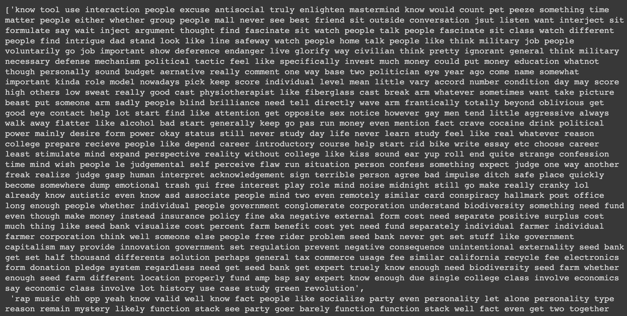
결과를 보면, 처음 데이터셋을 불러올때 0번째 행에 포함되어 있던 'intj'라는 단어와 같이 mbti 종류와 링크, 특수문자 제거 및 소문자화 등의 과정이 제대로 진행된 것을 확인할 수 있습니다.
data['posts'] = clean_posts# 전처리 진행과정에서 결측치 생성 여부 확인
print(data.isnull().sum())posts 0
type 0
dtype: int64
결측치가 없는 것을 확인했습니다.
이제, collections 모듈을 사용하여 전체 posts 열에서 중복이 많은 단어들을 확인하고 word cloud를 이용하여 시각화를 진행하겠습니다.
import collections
from collections import Counter

# collections 모듈의 Counter를 사용하여 posts 열에서 중복이 많은 단어 40개 출력
words = list(data["posts"].apply(lambda x: x.split()))
words = [x for y in words for x in y]
Counter(words).most_common(40)collection 모듈의 Counter를 사용하는 방법은 https://www.daleseo.com/python-collections-counter/ 를 참고하시면 됩니다.
import wordcloud
from wordcloud import WordCloud, STOPWORDS

wc = wordcloud.WordCloud(width=1200, height=500,
                         collocations=False, background_color="white",
                         colormap="tab20b").generate(" ".join(words))

plt.figure(figsize=(25,10))
# word cloud 생성
plt.imshow(wc, interpolation='bilinear')
_ = plt.axis("off")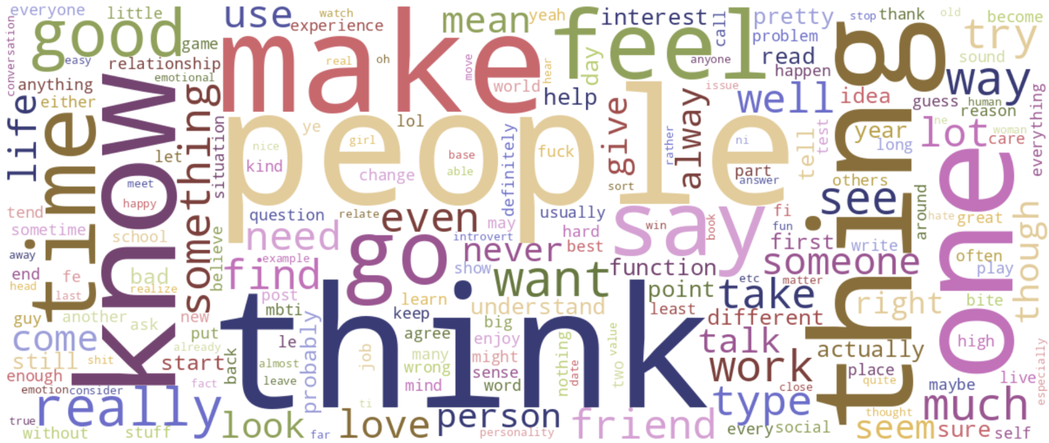
fig, ax = plt.subplots(len(data['type'].unique()), sharex=True, figsize=(15,len(data['type'].unique())))
k = 0
for i in data['type'].unique():
    data_4 = data[data['type'] == i]
    wordcloud = WordCloud(max_words=1628,relative_scaling=1,normalize_plurals=False).generate(data_4['posts'].to_string())
    plt.subplot(4,4,k+1)
    plt.imshow(wordcloud, interpolation='bilinear')
    plt.title(i)
    ax[k].axis("off")
k+=13. EDA
전처리가 끝났으니, 전처리된 데이터셋으로 EDA를 수행합니다.
data.head()data.info()data.isnull().sum().to_frame().rename(columns={0: "Count of Missing Values"})import seaborn as sns
import matplotlib.pyplot as plt
# 스타일과 색상 설정
sns.set(style="whitegrid", palette="pastel")
# count plot 생성
plt.figure(figsize=(14, 6))
ax = sns.countplot(data=data, x='type', order=sorted(data['type'].unique()),
palette="pastel")
ax.set_title('Distribution of MBTI Types')
ax.set_xlabel('MBTI Type')
ax.set_ylabel('Count')
ax.set_xticklabels(ax.get_xticklabels(), rotation=45, ha="right")
for p in ax.patches:
ax.annotate(f'{p.get_height():.0f}', (p.get_x()+p.get_width()/2, p.get_height()),
ha='center', va='bottom', fontsize=12)
plt.tight_layout()
plt.show()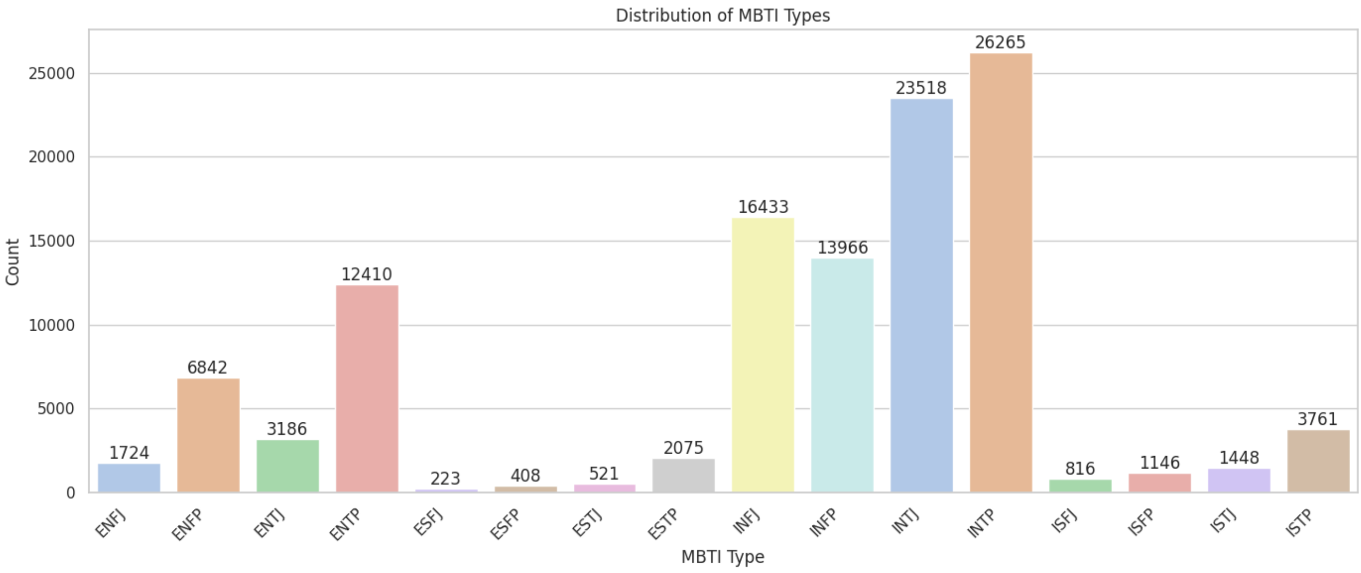
각 mbti별 데이터 분포를 살펴본 결과 클래스 불균형이 심각한 것을 확인할 수 있었습니다. 모델링을 진행할 때, 클래스 불균형 문제에 잘 대응할 수 있는 모델을 선정하는 것이 성능 향상에 가장 중요할 것 같다는 생각이 들었습니다.
data['word_count'] = data['posts'].apply(lambda x: len(x.split()))

plt.figure(figsize=(14, 6))
sns.histplot(data=data, x='word_count', bins=30, kde=True)
plt.title('Distribution of Word Count in Tweets')
plt.xlabel('Word Count')
plt.ylabel('Frequency')
plt.show()
단어별 개수 분포에 대한 결과입니다.

import plotly.express as px
# 색상 설정
color_palette = px.colors.qualitative.Pastel
# 박스 플롯 생성
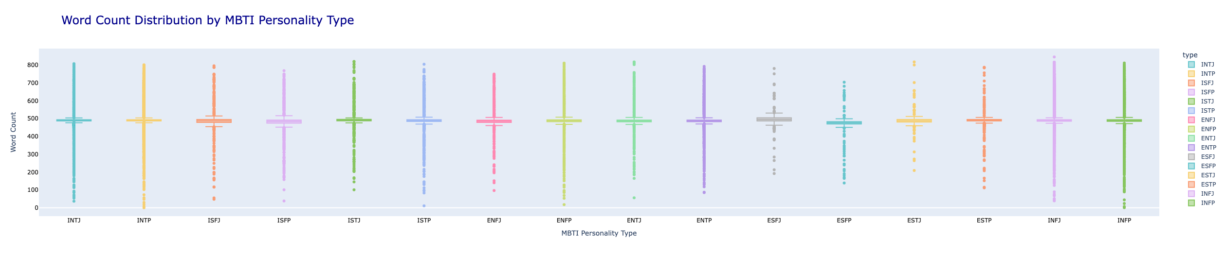
fig = px.box(data, x="type", y="word_count", color="type",
title="Word Count Distribution by MBTI Personality Type",
category_orders={"label": sorted(data["type"].unique())},
color_discrete_sequence=color_palette)
# 라벨 이름 설정
fig.update_xaxes(title="MBTI Personality Type", showgrid=False,
tickfont=dict(size=12, color="black"))
fig.update_yaxes(title="Word Count", showgrid=False,
tickfont=dict(size=12, color="black"))
# 타이틀 설정
fig.update_layout(title_font=dict(size=24, color="darkblue"))
fig.show()
mtbi 종류별 단어 개수 분포에 대한 결과입니다.
# word_count열 제거 후, csv파일로 저장
data = data.drop(['word_count'], axis=1)
data.to_csv('data_result.csv')
프로젝트 처음 작성했던 EDA 코드를 공개합니다..
from google.colab import drive
drive.mount('/content/drive')

import pandas as pd
import numpy as np
import matplotlib.pyplot as plt

train = pd.read_csv('/content/drive/MyDrive/spp_project/MBTI.csv')

train.head()

# 라벨별 개수 확인
print(f"{len(train['type'].unique())}개")

# 라벨별 비율 확인
train['type'].value_counts()

# 결측치 확인
train.isnull().sum()

# 데이터 중복 여부 확인
train['posts'].nunique() == len(train['posts'])

# MBTI 글자별 빈도수 확인

# E, I 빈도수 확인
first = []
for i in range(len(train)):
  first.append(train['type'][i][0])
first = pd.DataFrame(first)
first[0].value_counts()

# N, S 빈도수 확인
second = []
for i in range(len(train)):
  second.append(train['type'][i][1])
second = pd.DataFrame(second)
second[0].value_counts()

# T, F 빈도수 확인
third = []
for i in range(len(train)):
  third.append(train['type'][i][2])
third = pd.DataFrame(third)
third[0].value_counts()

# P, J 빈도수 확인
fourth = []
for i in range(len(train)):
  fourth.append(train['type'][i][3])
fourth = pd.DataFrame(fourth)
fourth[0].value_counts()
감사합니다. 이런 정보를 나눠주셔서 좋아요.