[2024 LLM Study] 4. Pretraining part.2

Minhan Cho·2024년 7월 25일

Architecture Choice

대부분 LLM들이 Causal decoder architecture를 사용하고 있으나, 이것이 진짜로, 왜 좋은지에 대해서는 많은 논의가 이루어지지 않았음
LM objective를 학습시키면서 causal decoder architecture는 zero-shot, few-shot generalization capacity가 학습되는 것으로 보임. 또한, 이후의 instruction tuning & alignment tuning과 causal decoder 모델의 궁합이 좋은 것으로 보임
causal decoder가 scaling law에 큰 영향을 받고, 따라서 computational budget, dataset size, parameter size를 늘림으로써 model capacity를 키울 수 있음. 다만, encoder-decoder architecture에서의 scaling law의 적용에 대한 연구는 적다는 것이 한계.

이번 survey 내용은 pretrain 시 상세한 configuration과 실제 모델들은 어떻게 학습됐는지를 중심으로 보여줌

Pretraining (cntd.)

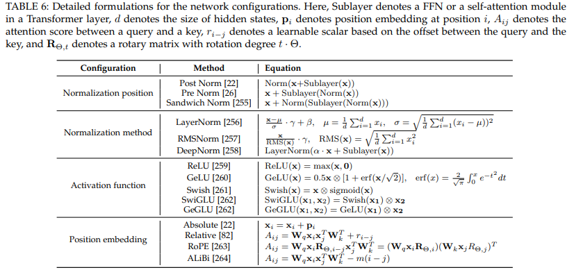
Detailed Configuration

summary: (1) RMSNorm을 layer normalization으로 사용하고, (2) SwiGLU 또는 GeGLU를 activation function으로 사용. (3) embedding layer 다음에는 layer normalization을 사용하지 말 것이며, (4) position embedding으로는 RoPE, ALiBi를 사용할 것

상세 내용
- Normalization Methods: 어떤 정규화 방법 (batch norm, layer norm etc.) 을 사용할 것인지?
- Normalization Position: normalization을 어느 단계에 적용할 것인지?
- Activation Functions: 어떤 activation function을 사용할 것인지?
- Position Embeddings: 어떤 방식의 position embedding을 사용할 것인지? position embedding이 잘 학습되지 않으면 long context에 대해 대응이 떨어질 수 있음
- Attention: 어떤 attention 방식을 사용할 것이고, 각각의 장점은 무엇인지?
  PyTorch의 범용 attention (FlexAttention)
- Pretraining Task: Pretraining의 objective를 무엇으로 설정할 것인지?
- Long Context Modeling: 긴 context에서 position embedding을 어떻게 설정할 것인지?
- Decoding Strategy: 어떤 방식의 decoding strategy를 설정할 것인지?

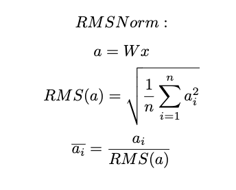
Normalization Methods

training instability 때문에 pretraining 단계에서 normalization이 사용됨 (LayerNorm in Transformer)

LayerNorm: BatchNorm이 초기에는 많이 사용되었으나, sequence length가 다양하거나 small batch data에서 부적합함. 따라서 layer마다 activation의 mean과 variance를 계산해서 re-center & re-scale하는 layernorm이 제안됨
RMSNorm: Gopher와 Chinchilla에서 사용된 normalization으로, activation sum의 root mean square만을 사용하여 학습 효율을 높임
DeepNorm: MS에서 제시한 normalization으로, 1000개 layer까지 확장 가능하여 stability & 성능을 향상함. GLM-130B에 적용됨.

Normalization Position

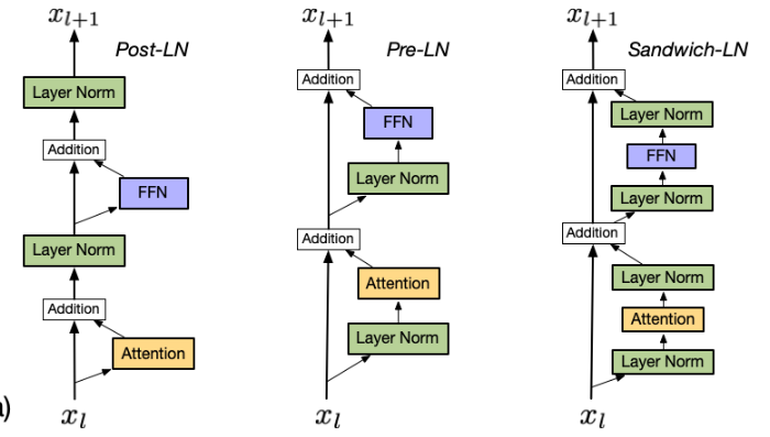
post-LN: vanilla Transformer에서 적용되었으나 output layer에서의 large gradient 때문에 instable한 것으로 밝혀져 사장됨.
pre-LN: sub-layer 이전, final prediction 이전에 normalization하여 stability를 높였으나, post-LN보다는 성능이 떨어지며, 100B 이상의 모델에서는 unstable 하다고 밝혀짐
sandwich-LN: pre-LN + residual connection (addition) 이전에 normalization 을 한 번 더 함. 이 경우, value explosion이 해결되기는 하는데, stability가 떨어져서 collapse of training이 발생하기도 함.

Activation Functions

ffn에서 GeLU가 많이 사용됨. SwiGLU같은 GLU 계열의 variant가 성능 향상을 위해 쓰이지만 GeLU와 비교해 parameter가 50% 가량 더 필요하다는 한계.

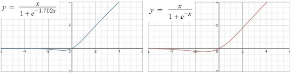
SwiGLU: Swish + GLU

Swish: $\beta$ 값에 따라 다른 특성을 갖는 activation function
$Swish(x) = x \cdot \sigma(\beta x)$
- $\beta$ 가 1이면 SiLU, 0이면 scaled linear function, inf이면 ReLU와 유사해짐
- 장점: (1) 0 보다 커도 cap이 없음 (2) 0보다 작을 때 0으로 수렴하기는 하나, 일부 정보가 남아있음 (3) differentiability (4) 단조증가하지 않음
GLU: componen-wise product of 2 linear transformation input
$GLU(x, W, V, b, c) = \sigma(xW+b) \otimes (xV+c)$

SwiGLU가 왜 더 좋은지 설명하기는 어렵지만, 어쨌거나 성능이 더 좋음 (물론 GLU 때문에 parameter가 많기는 함)

Position Embeddings

self-attention이 sequence의 순서에 영향을 받지 않으므로 (permutation equivariant) 토큰의 위치를 넣기 위해 사용됨

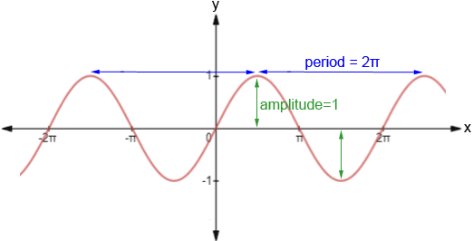
absolute position embedding: sinusoidal 함수값 (아래 fiugre 참조) 을 더하거나 position embedding을 학습해 더해줌. position embedding을 학습해 더해줄 경우, 학습 중에 참조하지 않은 더 긴 input에 대응하기 힘들다는 한계가 있음
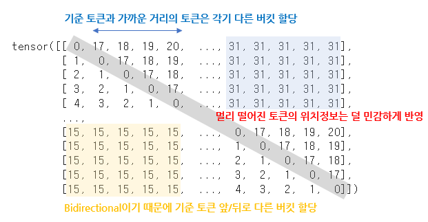
relative position embedding: learnable parameter를 attention에 추가해서 key와 query의 거리에 따라서 position이 학습됨 (T5, Gopher에서 도입). 가까운 거리의 token과는 거리를 민감하게 학습하고, 먼 거리의 token과는 거리를 덜 민감하게 학습

Rotary Position Embedding: input embedding에 rotation matrix를 적용하는데, sequence 내 토큰의 위치 & embedding dimension에 따라 결정됨

Attention

full attention: vanilla Transformer에서 사용된 모든 token 사이의 attention
sparse attention: full attention에서 quadratic computational complexity를 가지므로, query가 모든 토큰이 아닌, 일부 sequence에 대해서만 attention을 갖는 방식이 제안됨
Multi-query/grouped-query attention: MQA는 key와 value의 head를 하나로 통일 (different heads share the same linear transformation matrices) 하여 약간의 성능 하락과 큰 속도 향상을 기록 (StarCoder, PaLM), GQA는 head를 여러 개의 group으로 나눠 각 group 내부에서는 같은 matrix를 공유하는 방법 (LLaMA2)
FlashAttention: GPU를 더 효율적으로 사용하는 attention mechanism (pytorch에서 사용 가능)
PagedAttention: KV cache가 실제 inference에서 차지하는 메모리 및 시간이 큰데, k와 v를 잘라서 물리적으로 다른 메모리에 저장하여 속도를 향상

Pre-training Tasks

보통 language modeling과 denoising autoencoding을 pretraining task로 사용

Language Modeling

단, prefix decoder architecture에 사용되는 학습방법인 prefix decoder language modeling은 prefix token 개수만큼 학습에서 제외되므로 학습에 약간 부정적인 영향을 줌

Denoising Autoencoding

일부 span (tokens or words) 을 다른 span으로 바꿔치기해서 바뀐 span을 복원하는 것. 적용하기 복잡해서 LM task에 비해 많이 사용되지는 않지만, GLM-130B에서 사용된 바 있음.

Mixture-of-Denoisers

UL2 loss라고도 지칭되며, LM과 DAE objective를 각각 S-denoiser (LM), R-denoiser (DAE, short span & low corruption), X-denoiser (DAE, long span & high corruption)으로 세분화하여 학습. 학습할 때 special token ({R}, {S}, {X}) 를 가장 앞에 두어 각 denoiser에 학습될 수 있게 함. PaLM2에 사용.

Long Context Modeling

GPT-4 Turbo는 128k, Claude 2.1은 200k의 context window를 가지는데, 이는 scaling position embedding과 adapting context window를 통해 구현됨.

Scaling Position Embeddings

Direct model fine-tuning: 단순히 긴 텍스트에 학습. 최근 연구에서는 quality가 length보다 더 중요하다는 결과 & 너무 시간이 오래 걸린다는 결과도.
position interpolation: OOD rotation angle을 처리하기 위해 원래 length $L$ 을 target length $L'$ 에 대해 나눠 positional encoding으로 줌. direct finetuning보다는 효율적이지만 short text에서 성능 하락.
position truncation: OOD rotation angle 문제를 해결하기 위해 긴 길이의 텍스트를 truncation하거나 interpolation함.
base modification: 보통 고정된 context에 대해 LLM이 학습하게 되는데, 긴 텍스트에 대해서는 positional encoding을 충분히 학습하지 못한다는 한계가 있음. 따라서 RoPE 식에서 사용되는 b의 값을 조정하여 더 긴 텍스트에도 잘 학습되도록

Adapting Context Window

parallel context window: input text를 multiple segment로 나누어 각각 encode하고, decoding 할 때 각각의 segment를 참조. 단, segment의 순서를 구별할 수 없으므로 특정 태스크에서 성능 하락
$\Lambda$ shaped context window: LLM은 sequence의 처음과 끝에 가장 큰 attention weight를 준다는 결과에 근거 (lost in the middle phenomenon), attention weight가 높은 처음과 끝만 남기고 masking해서 학습. 단, long-range dependency가 있다는 한계
external memory: 소수의 token만으로도 대부분의 attention을 처리할 수 있음. 따라서, kNN을 사용하여 해당 토큰과 가장 가까운 k개의 token만을 사용하여 생성하는 것. 실제로 layer 하나만 kNN으로 token을 고르고, 나머지 layer에서는 normal context window를 사용

Decoding Strategy

pretraining 뒤, 우리가 원하는 output을 만들기 위해 decoding을 어떻게 할 것이냐?

greedy search

greedy search background

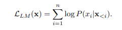
보통의 causal decoder architecture는 아래의 LM objective로 학습이 되므로,

$L_{LM}(x) = \sum^n_{i=1}logP(x_i|x_{<i})$

basic decoding strategy는 앞의 token들을 바탕으로 다음 step $i$ 에 나올 token을 예측하는 greedy search이며, 아래 식이 되겠음.

$x_i=argmax_xP(x|x_{<i})$

단, greedy search는 대부분의 text generation task에서 잘 작동하지만, 단순히 token 단위의 probability를 기준으로 next token을 선택하는 것은 전체 문장에서 higher probability를 갖지만 낮은 local estimation을 갖는 sequence의 생성을 방해하여 open-ended generation task (story generation, dialogue etc.) 에서 어색하거나 반복되는 문장을 내뱉는 경우가 있음 (ICLR 2020).

Beam Search: beam size (n) 개 만큼의 highest probability를 갖는 sentence를 계속 유지하여 최종 단계에서 가장 높은 probability를 갖는 sentence를 선택 (beam size가 1이면 greedy decoding과 동일). beam size는 3-6 정도로 하는데, beam size가 클수록 performance는 하락
Length Paenalty: beam search는 짧은 문장을 선택하게끔 하는 문제가 있어 length penalty를 부여하여 sentence length를 normalize함

sampling-based methods

greedy search에서 단순히 argmax인 token을 선택했다면, sampling-based methods에서는 token probability에 따라서 뒤의 토큰을 sampling하며, 식은 아래와 같음

$x_i \sim P(x|x_{<i})$

다만, 낮은 확률값의 개연성 없는 토큰이 선택될 수 있으므로, 다음과 같은 strategy를 선택하여 완화함

Temperature sampling: token probability에 temperature를 추가해서 softmax. temperature $t$ 가 높아지면 low probability의 단어가 선택되는 확률이 높아짐. $t$ 가 0일 때는 greedy search와 동일하고, 1이면 default random sampling이며, infinity이면 모든 단어의 확률분포가 uniform하게 됨

$P(x_j|x_{<i})=\frac{exp(l_j/t)}{\sum_{j'}exp(l_{j'}/t)}$ , $l_{j'}$ 는 token logit을 의미

Top-k sampling: top-k 개의 token만 sampling하여 사용
Top-p sampling (nucleus sampling): probability의 총합이 $p$ 인 token개수만큼 sampling

Decoding Efficiency Issues

decoder는 (1) prefill stage와 (2) incremental decoding stage로 나뉘는데, 전자가 후자보다 훨씬 많은 메모리를 잡아먹음

Model Training

important settings, tecniques, tricks for training LLMs에 대해 설명.

최근 GPT-4는 predictable scaling을 도입하여 smaller model을 학습시켜 large model의 performance prediction을 진행하도록 하여 시간과 자원을 줄였음.

Optimization Setting

batch training, learning rate, optimizer, training stability에 대해 서술

Batch Training: GPT-3, PaLM의 경우 32k에서 3.2M token까지 batch size를 dynamically 조정하여 training stability를 향상함
Learning rate: 대부분 0.1-0.5% 의 training step 동안 warm-up scheduling을 적용, lr의 최대값은 $5 \times 10^{-5}$ 에서 $1 \times 10^{-4}$ 정도. GPT3의 경우 $6 \times 10^{-5}$ 를 적용. training loss convergence까지 cosine decay를 적용하여 lr max value의 10% 정도를 reduce함.
Optimizer: Adam, AdamW (GPT-3) 를 보통 사용. hyperparameter로는 $\beta_1 = 0.9, \beta_2 = 0.95, \epsilon = 10^{-8}$ 사용. Adafactor (T5, PaLM)은 GPU 메모리를 죽이기 위한 Adam의 변형인데, $\beta_1 = 0.9, \beta = 1.0-k^{-0.8}$ ( $k$ 는 training step의 수) 로 설정.
Stabilizing the Training: model collapse까지 야기할 수 있는 training instability issue에 대응하기 위해 weight decay & gradient clipping을 사용하는데, gradient clipping은 1.0, weight decay는 0.1로 설정하는 게 보통임. 이외 PaLM이나 OPT는 training loss spike가 나면 이전 checkpoint를 불러와서 다시 학습한다든지, spike난 data를 제외하는 방식으로 대응하기도 하고, GLM은 embedding layer gradient를 축소시킴으로써 완화하려 하였음

Scalable Training Techniques

LLM이 너무 커서 GPU 메모리에 올라가지 않는 점에 대응할 수 있는 방안들

3D Parallelism

3D parallelism은 data parallelism, pipeline parallelism, tensor parallelism을 합한 것임. 실제로 8-way data parallelism, 4-way tensor parallelism, 12-way pipeline parallelism을 동시에 사용해 BLOOM을 384개 A100에 학습시킨 바 있음.
사용을 원한다면, DeepSpeed, Colossal-AI, Alpa에서 지원.

Data parallelism: 여러 개 GPU에 모델 파라미터와 optimizer step을 복사한 다음 corpus를 나눠서 학습. gradient는 합쳐져서 update한 뒤 update된 model parameter를 다시 복수의 gpu에 복사. data parallelism을 위한 코드가 쉽고 잘 갖춰졌다는 게 장점
Pipeline parallelism: 모델 layer를 복수의 gpu에 나눠서 처리하는 것인데, 이전 학습 처리 결과를 대기하면서 소요되는 시간 (bubbles overhead) 같은 문제가 있어, GPipe나 PipeDream에서는 multiple batch padding이나 asynchronous gradient update같은 것들을 적용함
Tensor parallelism: parameter matrices를 decomposing하여 복수의 gpu에 올리는 것. Megatron-LM에서 이를 지원하고, Colossal-AI는 이를 적용하였음. Transformer model에서 attention을 decompose 가능

ZeRO

DeepSpeed에서 제공하는 테크닉으로, data parallelism에서 발생하는 memory redundancy (같은 parameter, optimzer parameters, model gradients가 각기 다른 gpu에 저장되는 것)에 대응함. 각 GPU에는 데이터의 일부만 저장하고, 다른 데이터를 불러올 필요가 있으면, 다른 GPU에서 retrieve하여 communication overhead를 줄인다고. PyTorch에서 ZeRO의 변형인 FSDP를 지원함.

Mixed Precision Training

BERT같은 PLM에서는 32bit floating-point (FP32) 를 써서 학습시키는데, LLM에서는 FP16을 사용해 메모리 사용과 communication overhead를 줄임. 당연히 FP32보다는 accuracy가 낮아서 Brain Floating Point (BF16) 을 사용해 significant bits를 줄이고, exponent bits를 늘려 대응했다고 함.