Bi-Directional Attention Flow for Machine Comprehension (2017) a.k.a. BiDAF

0. Abstract

• Machine Comprehension(MC)은 Machine QA와 같음: context와 query간 복잡한 interaction 필요
• 최근(2017)까지 attention은 MC에도 많이 확장되었는데,
  - context의 작은 부분에 집중하여 fixed-size vector로 요약하거나,
  - couple attentions temporally(?),
  - uni-directional atention을 구성하는 등의 노력이 있었음
• 본 논문에서는 Bi-Directional Attention Flow(BiDAF)를 제시함
  - 본 모델은 multi-stage(hierarchical) 구조로, context를 다양하게 표현하는 모델임(represents the contet at different levels of granularity)
  - bi-directional attention flow mechanism을 사용하여 query 중심의 context representation을 만들 수 있음(이전에는 summarization이 필요하였음)
• 본 모델은 SQuAD와 CNN/DailyMail cloze test에 대해 SoTA 달성

1. Introduction

• 최근 Machine Comprehension(MC)와 Question Answering(QA) 부문의 발전은 neural attention mechanism을 사용함으로써 가능하였음
  - attention이 하는 일은 무엇인가? context 또는 image에서 질문에 가장 연관 있는 부분에 집중할 수 있도록 함
• 이전에 사용되었던 attention은 다음과 같은 특성을 갖고 있었음
  1. 사전에 계산된 attention weight을 context에 적용해서 fixed-size vector로 표현하고(summarization), 질문과 연관있는 정보를 추출함
  2. attention이 temporally dynamic하게 사용되는데, 이는 다시 말해 이전 time step의 attention이 현재 time step의 attention weights 계산이 영향을 준다는 것
  3. 이전의 attention은 uni-directional: 보통 query를 context paragraph 또는 image patch에 대보는(attends) 형식
• 본 논문에서는 Bi-Directional Attention Flow(BiDAF)를 제안하는데, 이는 다양한 관점에서 context를 분석하여 만들어진 representation을 이용함: character-level, word-level, contextual embeddings
• 위의 granularity에서 bi-directional attention flow를 사용해 query-aware context representation을 만듦(query-to-context representation이 아닌 이유는 query-to-context, context-to-query attention이 사용되기 때문)
• 본 mechanism은 이전의 attention에 비해 다음과 같은 개선점이 있음:
  1. 본 논문의 attention은 fixed size vector(summarization)를 만드는 데에 사용되지 않음: time step마다 attention이 계산되어 다음 layer로 전달되며, 정보 손실을 막음
  2. memory-less attention mechanism 사용: Bahdanau et al. (2015)에서는 attention을 반복적으로 계산했는데(dynamic attention), 본 연구에서는 각 time step의 attention은 현재 time step의 query와 context 간의 계산일 뿐
     이후 attention간의 interaction 계산은 modeling layer로 넘겨버림으로써 시간을 줄일 수 있었음
     또한, 이런 식으로 attention mechanism을 짠 것(이전의 attention을 고려하지 않는 것)은 이전 time step에서 잘못된 attention이 학습에 반영되는 것을 막을 수 있음
     시간 뿐 아니라 성능도 향상
  3. attention을 query-to-context, context-to-query 양방향으로 사용함으로써 서로에게 complimentary information을 제공할 수 있음
• BiDAF 모델이 SQuAD, CNN/DailyMail cloze test에서 SoTA 달성

2. Model

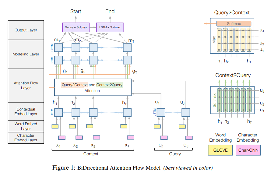
Character Embedding Layer (CNN) + Word Embedding Layer (GloVe) + Highway Networks
-> Contextual Embedding Layer (LSTM)
-> Attention Flow Layer
-> Modeling Layer (bi-LSTM)
-> Output Layer
참고: $H_{:t}$는 $H$의 $j$-th column이라는 notation

(1) Character Embedding Layer

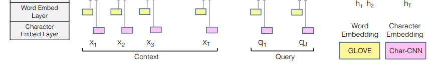
• Yoon Kim, Convolutional neural networks for sentence classification, 2014에서 아이디어 따왔음
• word를 character 단위로 쪼개고 CNN 넣어서 max-pooling 진행, output은 모든 단어마다 fixed-size vector가 되도록

(2) Word Embedding Layer

• pretrained GloVe 사용
• (1)의 character CNN과 (2)의 GloVe를 concatenate해서 two-layer Highway Network(Srivastava et al., 2015.)로 올려보냄
• Highway Network까지 다 거진 document와 query의 shape은 각각 d-dimension $\times$ document 단어 개수(또는 query 단어 개수)
  context: $X \in R^{d \times T}$ query: $Q \in R^{d \times J}$

Highway Networks?

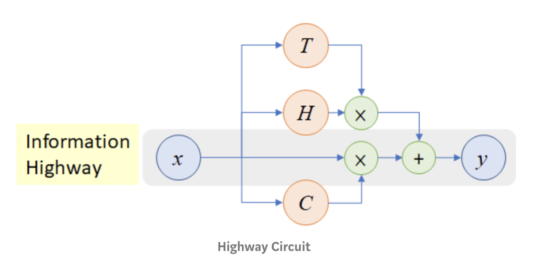
• Rupesh Kumar Srivastava, Klaus Greff, and Jurgen Schmidhuber. Highway networks. arXiv preprint arXiv:1505.00387, 2015. (extended abstract), full paper
• 원래는 visual 쪽에서 제안된 모델
• LSTM에서 영감을 받아 gating units를 사용, 어떤 정보는 gate를 거치고, 어떤 정보는 그대로(without attenuation) 다음 layer로 전달됨
• highway network는 중첩 정도와 관계없이 optimization 가벼움(900개까지 중첩되어도 SGD with momentum으로 optimization 가능), 이는 layer 갯수가 늘어나면 훈련 비용이 늘어났던 기존 모델들에 비해 큰 장점

  $y = H(x, W_H)$: plain feed forward network ($H()$: affine transformation)
  $y = H(x, W_H) \cdot T(x, W_T) + x \cdot C(x, W_c)$: Highway Networks

• $T$: transform gate, input을 얼만큼 '변형($H()$: fc layer)된 형태로' 전달할 것인지
  $C$: carry gate, input을 얼만큼 '그대로' 보낼 것인지
  $C + T = 1$이 되도록 $C$와 $T$를 설정

(3) Contextual Embedding Layer

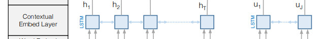
• bi-LSTM을 사용하여 embedding의 순서적 측면을 반영하도록 함: 결과는 2*d-dimension $\times$ document terms (또는 query terms)
  context: $H \in R^{2d \times T}$ query: $U \in R^{2d \times J}$
• character level(character embedding), word embedding(GloVe), context embedding(LSTM)은 다른 level에서 query와 context를 이해하고자 하는 시도임

(4) Attention Flow Layer

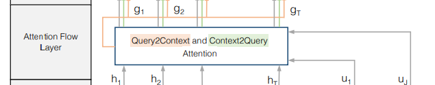
• context와 query의 정보를 연결(linking)하고 합치는(fusing) 과정
• 이전에 사용되었던 attention mechanism(Weston et al., 2015; Hill et a;, 2016; Sordoni et al., 2016; Shen et al., 2016)에서는 attention이 query와 context를 하나의 feature vector로 줄이는 것이 주요한 작업이었음
• 본 연구의 attention의 경우, 매 time step마다 attention vector가 이전 layer의 embedding 정보와 함께 다음 layer로 넘어감
  이는 이전 모델들과 비교하여 정보 손실을 줄일 수 있음
• (3)의 $H$(context representation)와 $U$(query representation)을 input으로 받아, context에 대해 query word level로 이루어져있는 행렬 $G$임
• attention layer에서 2가지 attention을 계산: from-context-to-query, from-query-to-context
  위 두 matrices는 similarity matrix $S \in R^{T \times J}$에서 계산될 수 있는데, $S_{tj}$는 $t$-th context word와 $j$-th query word의 similarity임
• 그렇다면 similarity이자 attention vector인 $S_{tj}$는 어떻게 구하느냐?

  $S_{tj} = \alpha(H_{:t}, U_{:j}) = \alpha(h, u) = w^T_{(S)}[h;u;h \circ u]$
  $H_{:t}, U_{:j}$는 각각 $t$-th, $j$-th column을 의미하며,
  $\circ$는 element-wise multiplication을, $h, u, h \circ u$는 각각 $2d$-dimensional vector이므로 $w_{(S)}$는 $6d$-dimensional trainable weight vector임

Context-to-Query(C2Q) Attention

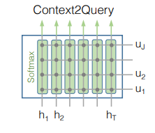
• C2Q attention은 해당 context word에 전체 query words 중 어떤 query word가 가장 relevant한지를 의미
  $a_t \in R^J$: $t$-th context word에 대한 query words의 attention weights($J$는 query vector의 차원임을 기억)
  $a_t = softmax(S_{t:}) \in R^J$로 계산되므로, 각각의 $t$에 대해 $\sum a_{tj} = 1$: '각각의 context word에 대해' query words의 attention weights의 합은 1
• $t$-th context word에 해당하는 query words의 attented query vector인 $\tilde U_{:t}$는 다음과 같이 계산될 수 있음
  $\tilde U_{:t} = \sum _j a_{tj}U_{:j}$
  따라서 $\tilde U \in R^{2d \times T}$임... 왜????

Query-to-Context(Q2C) Attention

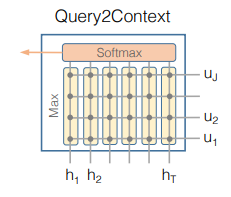
• Q2C attention은 해당 query word에 대해 전체 context words 중 어떤 context word가 가장 relevant 한지를 판단: 질문에 답하기 위해서는 문장의 어떤 단어가 가장 중요하냐?
  $b = softmax(max_{col}(S)) \in R^T$: $max_{col}$은 row-wise로 계산(performed across the column)
  query word에 대해 context에서 가장 중요한 단어의 가중치를 의미하는 attended context vector $\tilde h$는 다음과 같이 계산될 수 있음:
  $\tilde h = \sum_tb_tH_{:t} \in R^{2d}$
  $\tilde h$는 row만큼 반복되므로 $\tilde H \in R^{2d \times T}$
• contextual embeddings($H$), attention vectors($\tilde U, \tilde H$)를 이용해 $G$를 만들 수 있음: $G$의 column은 각각의 context word에 대한 query representation이라고 할 수 있음

  $G_{:t} = \beta (H_{:t}, \tilde U_{:t}, \tilde H_{:t})$
  위 식에서 $G_{:t}$는 $t$-th context word에 해당하는 column, $\beta$는 세 vector는 합치는(fuses) trainable vector function임
  $\beta$는 여러 방법으로 구현(e.g. multiple dense layer)할 수 있지만, 가장 좋은 방법은 simple concatenation이었음($\beta(h, \tilde u, \tilde h) = [h; \tilde u; h \circ \tilde u; h \circ \tilde h] \in R^{8d \times T}$)

(5) Modeling Layer

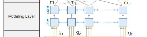
• 2개 layer의 bi-LSTM 사용, 각각 layer의 direction마다 $d$-dimensional
• modeling layer의 input은 $G$: 각각의 context word에 대한 query representation
• modeling layer의 output: query가 주어졌을 때 context words의 interaction을 포착하는 것(query가 조건으로 주어졌다는 점에서 contextual embedding layer와 다름)
  실제로는 $M \in R^{2d \times T}$이 튀어나와 output layer로 들어감: M의 각 column은 전체 context paragraph와 query와 관련한 'word'의 contextual information을 가짐

(6) Output Layer

• 실제 task가 무엇이냐에 따라 그 형태가 바뀔 수 있음: QA task와 cloze-style task에 따라 layer가 달라짐
• QA task는 정답으로 paragraph에 포함되어 있는 relevant sub-phrase를 찾아내는 것이며, 'sub-phrase'는 paragraph 내에서 '시작점(start index)'과 '종말점(end index)'를 찾아내는 것임
  • start index $p^1$은 다음과 같이 나타낼 수 있음: $p^1 = softmax(w^T_{(p^1)}[G;M])$
    $w_{(p^1)}$은 $[G;M]$이 10d차원(8d+2d)이므로 $w_{(p^1)} \in R^{10d}$인 trainable weight vector
  • end index를 구하기 위해 M을 또다른 LSTM에 넣어 $M^2 \in R^{2d \times T}$로 만들고, $p^2 = softmax(w^T_{(p^2)}[G;M^2])$과 같이 계산하여 end index에 대한 probability distribution을 계산

Training

• loss 계산: $L(\theta) = -\frac {1}{N} \sum_i^Nlog(p^1_{y^1_i} + log(p^2_{y^2_i})$을 minimize
  $\theta$는 모델 내 모든 trainable weights, $N$은 dataset의 크기(갯수), $y^1_i$와 $y^2_i$는 각각 true start index와 true end index, $p_k$는 vector $p$의 $k$-th value

Test

• 모델은 (k, l)을 span하며, k가 start index, l이 end index임
• $p^1_kp^2_l$의 maximum value일 때 해당 (k, l)이 반환

3. Related Works

Machine Comprehension

• Neural Machine Comprehension(MC)의 발달은 large dataset의 구축으로부터 시작되었음
  • MCtest(2013): 너무 작음
    -> Massive cloze test datasets(CNN/DailyMail, 2015) & Childrens Book Test(2016): neural MC의 시작
    -> Stanford Question Answering(2016): question 크기 100,000 이상
• 이전 end-to-end MC가 attention을 사용하던 방식:
  1. Bahdanau et al. (2015): "dynamic attention mechanism", query와 context, previous attention이 주어졌을 때 attention weights가 update됨(? 다시 한 번 정리해보자)
     -> BiDAF는 memory-less attention mechanism 사용
  2. Kadlec et al. (2016): attention weight을 한 번만 계산해서 output layer에 예측 위해 삽입
     Cui et al. (2016): Attention-over-Attention model, query와 key 사이의 2D similarity matrix 사용해 query-to-context attention을 계산
     -> BiDAF는 attention layer를 따로 정의하지 않고 RNN layer와 합쳐지도록 설계하였음
  3. Weston et al. (2015): 복수의 layer에서 query-context attention vector를 반복적으로 계산(multi-hop)

Visual Question Answering

• 초창기 VQA는 RNN으로 query를 encoding, CNN으로 이미지를 encoding한 후 둘을 합쳐서 답을 찾는 방식이었음
• attention이 도입된 이후, image patch에 query를 대보거나, query의 단어 단위로 image patch에 대조해서 높은 attention value를 가진 image patch가 답으로 제출되는 방식이 사용되었고, query를 unigram, bigram, trigram 등 multiple level로 표현하여 사용하기도 하였음
• attention matrix를 만드는 방식: element-wise product, element-wise sum, concatenation, Multimodal Compact Bilinear Pooling 등
• query를 image patch에 대조하던 기존 방식과 달리, image를 query word에 대조하는 방식도 등장하였음
  • 본 논문에서도 이 방식을 일부 차용하였으나, 본 논문은 attention flow가 RNN으로 되돌아간다는 점에서 차이가 있음

Machine Comprehension Previous Papers 조금 더 자세한 설명

• Bahdanau et al. (2015): Machine Translation에 attention이 등장했던 바로 그 역사적인 논문(이미 Machine Translation part에서 다루었음)
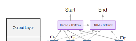
• Attention Sum Reader Kadlec et al. (2016), 보충자료
  

단순하게, query(question)을 bi-GRU 통과시켜 나온 representation을 각 단어의 representation과 dot product 한 것! 이후 softmax 이용해 정답일 확률이 가장 높은 단어를 뽑아낸다!

1. query representation, document 내의 word를 representation으로 구성
2. query representation과 document 내의 word representation(candidate answer) dot product해서 가장 확률이 높은 단어를 answer로 선정

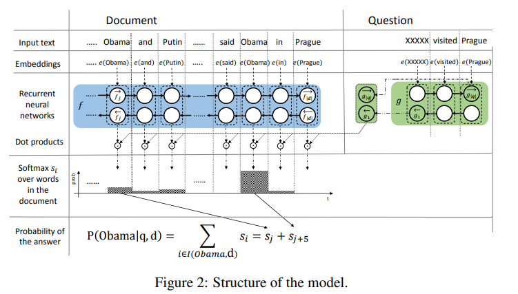
• Attention-over-Attention model Cui et al. (2016):
  

  1. document representation과 query representation을 dot product해서 document $\times$ query matrix("pair-wise matching matrix") 만들고
  2. column-wise softmax: query word에 대한 document level의 attention("query-to-document attention")
  3. row-wise softmax: 각 document term에 대해 query level의 importance 확인("importance distribution", "reversed attention", "document-to-query attention")
     row-wise softmax한 matrix를 column-wise average해서 "averaged query-level attention"을 생성
  4. 2의 column-wise softmax한 matrix와 3의 averaged query-level attention을 내적해 "attended document-level attention"을 생성
     이같은 dot product는 각각의 document-level attention(2에서 구했던 matrix의 column)을 query word 만큼의 가중치 줘서 계산하는 것과 같음
  5. prediction level에서 'sum attention'을 사용해 vocabulary 집합 내의 단어를 선택(상단의 Kadlec et al. (2016)에서는 document 내의 단어 중 하나를 선택하게 되어있음)
     sum attention?: 별 거 아님. 그냥 실제로 같은 단어인 경우 해당 term의 probability를 더한 값으로 prediction 하겠다는 것

MemNN(multihop)
Weston et al., 2015, Hill et al., 2016 등등 많이 사용되었던 모델

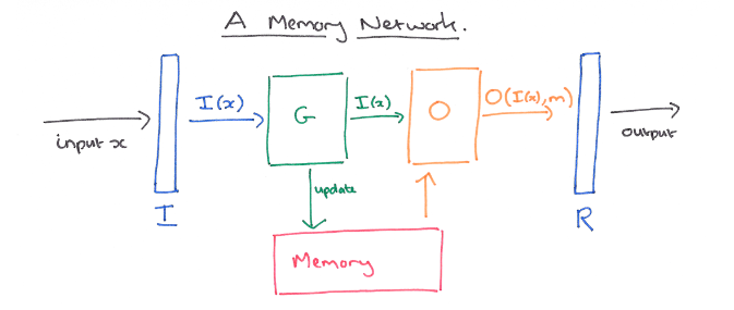
• 위와 같은 꼬리물기 하는 문장이 여러 개 나오는 QA에서 질문에 대한 답과 근거가 되는 문장을 annotation한 dataset에서, 모델도 새로운 문장(+이전에 있었던 query와 가장 유사도 높았던 문장)과 query와의 유사도 계산을 통해 문장을 계속 update
• annotation 힘드니까 이걸 soft alignment(attention)으로 만들어버린 게 end-to-end attention

4. Question Answering Experiments

SQuAD (Rajpurkar et al., 2016)와 해당 데이터에 모델을 적용한 결과를 서술

Dataset

• SQuAD는 Wikipedia를 사용한 data로, 100,000개 이상의 질문으로 구성되어 있음
• 질문에 대한 답은 '항상 context 안에 존재'
• model이 예측한 답과 사람이 쓴 답과 같으면 credit을 따는 방식
• metric: Exact Match(EM) & F1 score
  • F1 score는 글자 단위(character-level)에서의 precision & recall rate을 가중평균 한 것
• train 90k / dev 10k / unknown number of hidden test set

Dataset에 대한 사족

• SQuAD 1.x와 SQuAD 2.0의 차이는 'unanswerable question'이 없느냐(SQuAD 1.x)와 있느냐(SQuAD 2.0)의 차이임 https://rajpurkar.github.io/SQuAD-explorer/
  • squad 1.1
    
  • squad 2.0: SQuAD 1.1에서 가져온 100k q's + 50k unanswerable q's
    
• SQuAD 외에 다른 Machine Comprehension Dataset이 궁금하다면?: Dzendzik, D., Vogel, C., & Foster, J. (2021). English machine reading comprehension datasets: A survey. arXiv preprint arXiv:2101.10421.

Model Details

• paragraph와 question의 tokenizer는 PTB tokenizer, 정규표현식 기반의 word tokenizer임
• character level CNN의 1D filter는 100개, width 5
• hidden state size($d$): 100
• model parameters: 2.6 mln
• optimizer: AdaDelta
• batch size: 60
• (initial) learning rate:0.5
• number of epochs: 12
• drpoout rate: 0.2(CNN, LSTM, softmax 이전의 fc layer)
• moving averages of weights decay: exponential, 0.999 (raw weights 대신 moving averages가 test set에 사용됨)
• 훈련 시간 20h on Titan X GPU
• ensemble 모델 하나 더 설정: architecture, hyperparameters는 똑같이 고정하고 12 training runs 돌려서, 각 질문에 대해 highest sum of confidence scores 나온 answer를 선택

Results

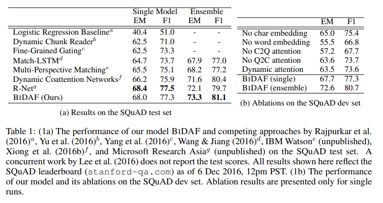
• BiDAF(ensemble)이 EM score 73.3, F1 score 81.1로 SoTA 달성 (table 참조)

Ablations

• char-level, word-level embeding이 모두 performance에 영향
• word embedding은 semantic에 강점이 있고, character embedding은 OOV나 rare word에 강점이 있음: 이는 이미 FastText, charCNN에서 한 번 짚은 바 있음
• bidirectional attention(attention 2번 쓴 것)의 효과를 측정하기 위해 Query-to-Context(Q2C)와 Context-to-Query(C2Q) attention을 각각 제거하고 실험해보았음
  • C2Q ablation study를 위해 C2Q(attended question vector $\tilde{U}$) 대신 query의 LSTM output average를 사용하였음
    C2Q는 metric 2가지에서 모두 10점을 떨어뜨리는 결과
  • Q2C ablation study를 위해 $G$가 $\tilde{H}$를 반영하지 않게 하였음
• 이전 attention model에서 사용되었던 dynamic attention model을 사용한 결과, 본 모델(static attention)이 3점 정도 더 나았음
  attention layer를 분리함으로써 attention layer 전에 있었던 4개 layer에서 나온 rich feature가 조화롭게 통합되었다고 추측할 수 있음
• Appendix B에는 $\alpha$와 $\beta$의 식을 다르게 구성하여보았음
  

Visualization

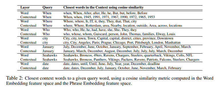
• when, where, who 같은 단어는 word embedding만 거치면 해당 단어가 무엇을 지칭하는지 모델이 잘 파악하지 못하지만, contextual embedding을 지나면 극적으로 달라짐(각 row의 위가 word embedding만 거쳤을 때, 아래는 contextual embedding까지 거쳤을 때)
  

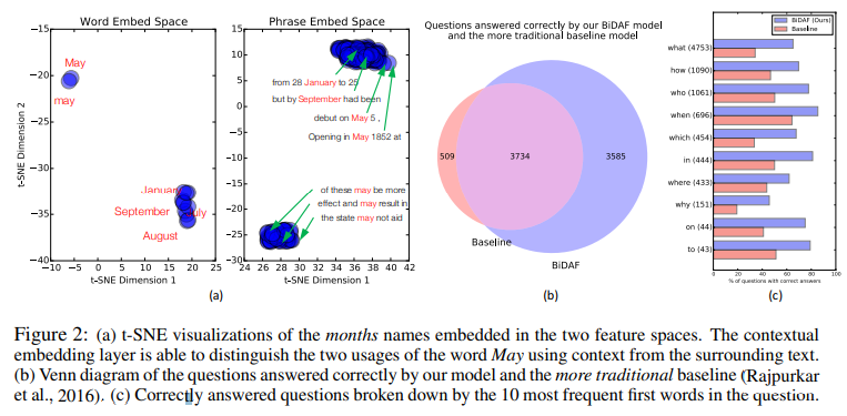
• t-SNE으로 나타냈을 때에도, word embedding만 거치면 'May'가 다른 월들을 지칭하는 단어들과 동떨어져 있는데, contextual embedding을 거치면 May의 사용법이 구별됨
  

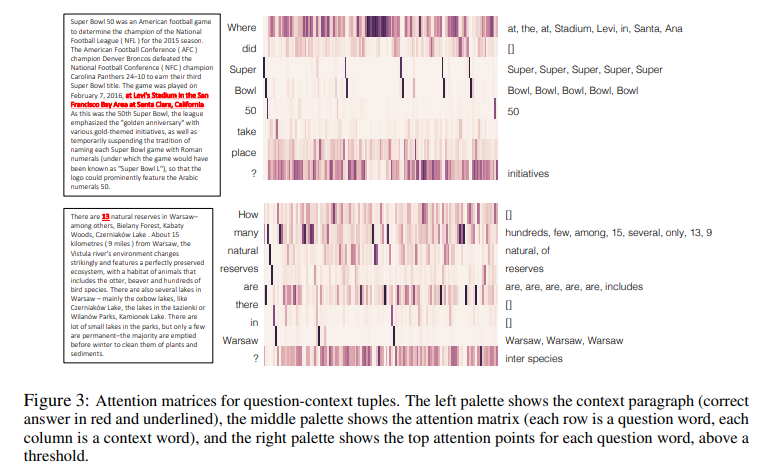
• attention matrices를 시각화한 결과, query에 매칭되는 context의 단어들을 확인할 수 있었음

Discussions

• baseline 모델이 정확하게 분류한 question의 86%를 본 모델 또한 정확하게 분류하였는데, 오답이 나온 14%는 clear patten이 없는 경우였음

Error Analysis

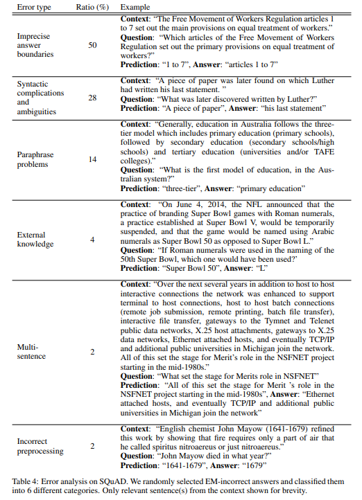
• EM 결과에서 틀렸던 50개 문제들을 뽑아서 6개 카테고리로 분류한 결과, 50%는 answer의 boundary가 불분명한 경우, 28%는 문법적으로 어렵거나 문법적으로 모호한 경우, 14%는 paraphrasing problems, 4%는 외부 지식(external knowledge)이 필요한 경우, 2%는 대답에 복수의 문장이 필요한 경우, 2%는 tokenizing 과정에서의 오류에 기인하였음을 파악할 수 있었음(Appendix A)

5. Cloze Test Experiments

CNN dataset, Daily Mail dataset을 이용해 cloze-style test를 진행하였음

Dataset

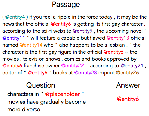
• cloze test: passage가 주어지고, 구멍 뚫어놓은 단어를 채워넣는 형태의 task
• train/dev/test: 300k/4k/3k(CNN) and 879k/65k/53k(DailyMail)
• 뉴스 기사가 주어지고, 해당 기사를 바탕으로 사람이 손으로 작성한 요약 문장에 구멍을 뚫어놓고 문장 완성
• 일반 단어라면 language modeling이 되어버릴테니(BERT 등 학습할 때 MLM 방식이랑 똑같음), 채워야 하는 단어는 항상 named entity & random ID로 익명화하였음, ID는 계속 바뀌도록 하였음

Model Details

• SQuAD와 거의 비슷하긴 한데, output layer에서만 조금 달라짐
  • cloze test는 한 단어 채워넣기 task이므로 start index($p^1$)은 필요하나, end index($p^2$)는 필요없으므로 loss 계산에서 후자는 지워짐
  • prediction layer에서는 non-entity words를 모두 제거해서 possible answer만 남겨둠
  • SQuAD와 달리 context paragraph에서 정답이 여러 번 등장할 수 있어서 같은 단어(entity)에 해당하는 $p^1$ probability를 모두 더한 probability distribution에서 최종 답안을 선택
• batch size 48, epoch num 8, validation data accuracy가 떨어지기 시작할 때 early stop
• Hill et al. (2016)에서 window-based method 따와 기사를 entity 주위 19개 단어 단위의 short sentence로 분할

Results

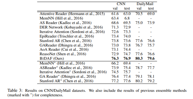
• CNN/DailyMail dataset에 대해 SoTA 달성

Conclusion

• BiDAF는 context를 다른 granularity에서 representation 만들고, bi-directional attention flow mechanism 쌓아 summarization 없이도 query 중심의 context representation 구성
• SQuAD, CNN/DailyMail cloze test에서 SoTA 달성
• ablation study에서는 모델의 모든 부분이 중요함을 보였음