15. Object Detection

• Approaches
  • Two-stage model
    consists of a region proposal module and a recognition module
    • R-CNN, Fast R-CNN, Faster R-CNN
  • One-stage model
    removes the proposal generating module and predicts object positions directly
    • YOLO, SSD, DETR

15.1. Two-stage model

15.1.1. R-CNN

(참고: zzwon1212 - R-CNN)

• Stage 1: Region proposals

  • extract ~2k region proposals using selective search.

• Stage 2: Object recognition

  • extract feature map using CNN from each proposal.
  • classify the feature vector
  • regress the feature vector

• Why R-CNN?

  • First modern deep learning based image detection
  • Significantly reduced computation from the brute-force method
  • Detection performs okay

• Why NOT R-CNN?

  • Computationally expensive
    • region proposal
    • ~2k independent CNN forward passes for each proposal

15.1.2. Fast R-CNN

(참고: zzwon1212 - Fast R-CNN)

• Stage 1: Region proposals

  • same as R-CNN

• Stage 2: Object recognition

  • extract (shared) feature map using CNN from one entire image
  • apply RoI Pooling Layer
    • projects each proposal onto shared feature map to get own feature map
    • apply max-pooling to own feature map to get fixed-length feature vector
  • classify and regress the feature vector using fc layers
    
    

• Why Fast R-CNN?

  • Better accuracy than R-CNN
  • 8~18x faster trainig time than R-CNN
  • 80~213x faster inference time than R-CNN
  • Much less memory space needed

• Why NOT Fast R-CNN?

  • Still using an off-the-shelf region proposal, which is computationally expensive. This is the main bottleneck of Fast R-CNN.

### 15.1.3. Mask R-CNN

- RoIAlign
Instead of simply taking max over uniformly split RoI, use linear interpolation to better estimate feature values at each cell.

15.1.4. Faster R-CNN

• Stage 1: Training RPN (Region Prposal Network)
  
  
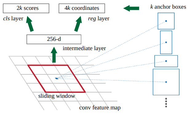
  • For each position in the last shared conv feature map, suppose a set of candidate bounding box called anchor.
  • We will predict 2 scores (object or not) and 4 coordinates for each anchor.
  • apply $n \times n$ convolution on the conv feature map to get new feature map with 256 channels.
  • apply two separate $1 \times 1$ convolution on the new feature map to get cls feature map with 2k channels and reg feature map with 4k channels.
  • Each position in cls feature map and reg feature map has scores and coordinates for $k$ anchors for that position.

• Stage 2: Same as Fast R-CNN

  • Using the RPN trained in Stage 1, perform RoI pooling, classification, and regression.

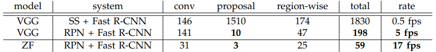
• Why Faster R-CNN?
  

15.2. One-stage model

15.2.1. YOLO

(참고: zzwon1212 - YOLO)

15.2.2. SSD

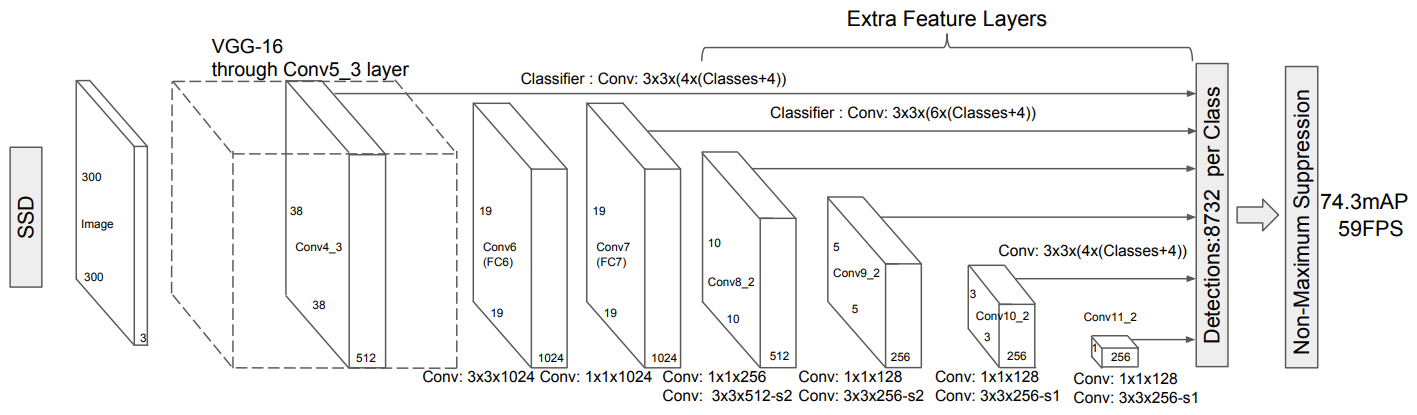
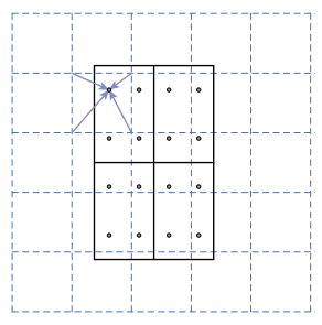
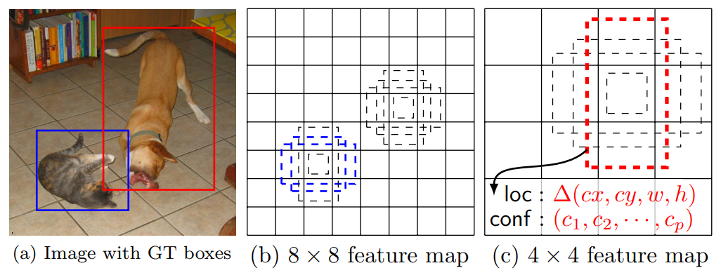
• Main idea

  • Each cell in earier conv layer looks narrow range of the image. So it can detect small objects.
  • Each cell in later conv layer looks wider range of the image. So it can detect large objects.

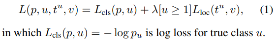
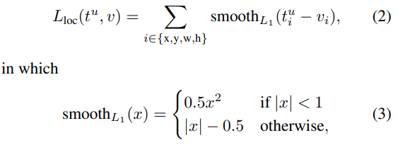
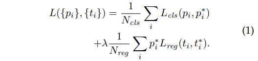
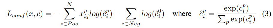
• Loss
  

  

  

• Results
  

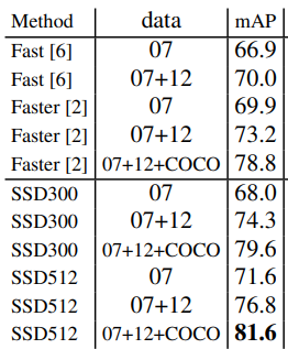
  • Accuracy: Fast R-CNN < Faster R-CNN < SSD
    
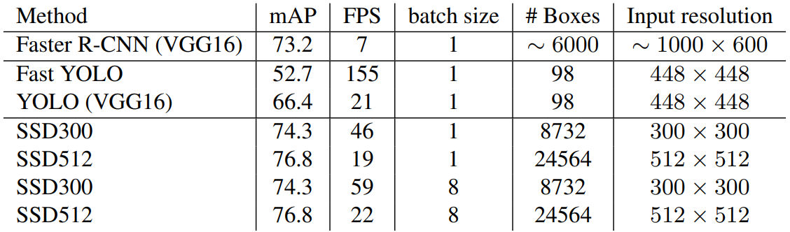
  • FPS: Faster R-CNN < SSD < YOLO

15.3. Transformer-based Approach

15.3.1. DETR (Detection Transformer)

• Main idea

  • A set-based global loss that forces unique predictions via bipartite matching.
  • Removing the need for many hand-designed components like a NMS.

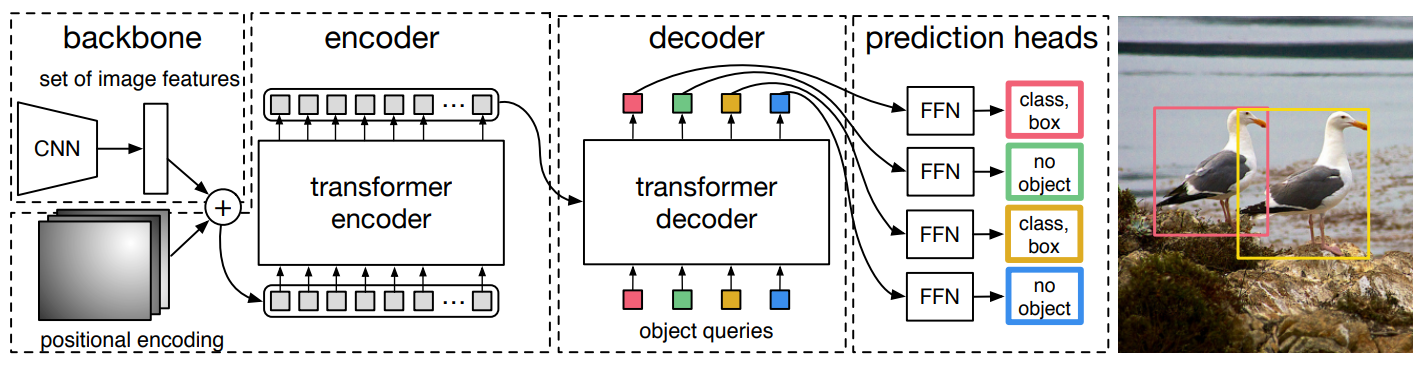
• Architecture
  

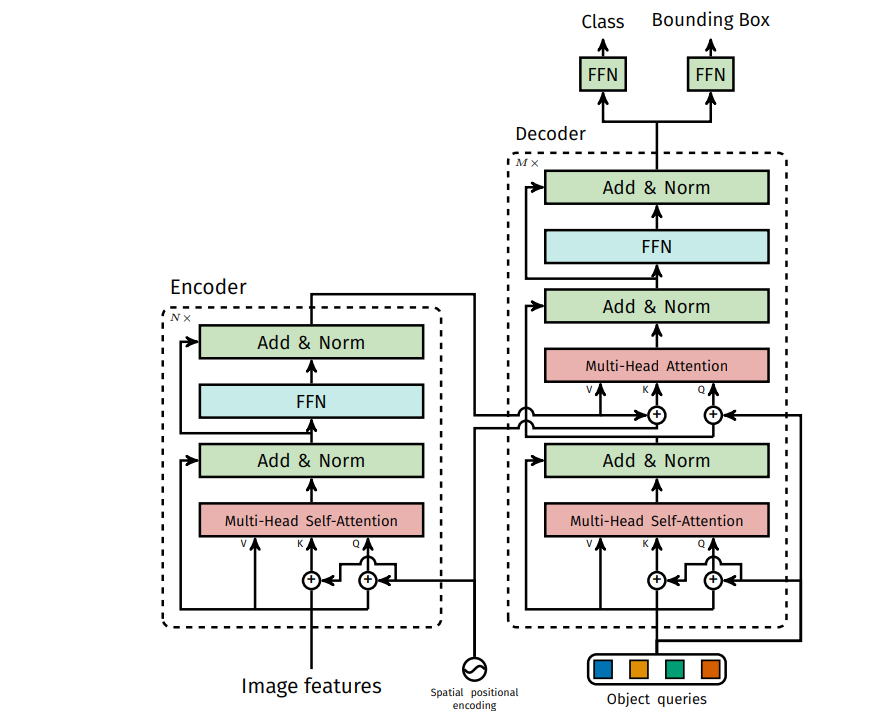
  • A CNN backbone extracts spaital features: $7 \times 7 \times 512$
  • Fixed positional encoding for each location (sinusoidal)
  • For spatial features as input tokens, a Transformer encoder contextualizes them throughout the entire image.
  • Starting from object queries (learnable positional encodings), a Transformer decoder outputs embeddings corresponding to the objects to be detected in the image.
  • Through fully-connected layers, each object embedding is mapped to its class and bounding box coordinates.

• Difference from the original Transformer

  • Outputs are produced in parallel, as opposed to autoregressive manner. This is because there is no obvious order between objects in the image.
  • Positional encoding is applied only to the queries and keys.
  • Positional encoding is added at every layer. (No proof but experimental evidence)

• Training

  • Because there is no natural order among objects in the image, we actually do not know which box is for which object. How should we score a prediction when we compute loss?
  • DETR infers a fixed-size set of $N$ predictions, wher $N$ is significantly larger than typical number of objects in an image.
  • Suggested solution: an optimal bipartite matching between predicted and ground truth objects is performed, then object-specific bounding boxes are optimized independently.

• Results

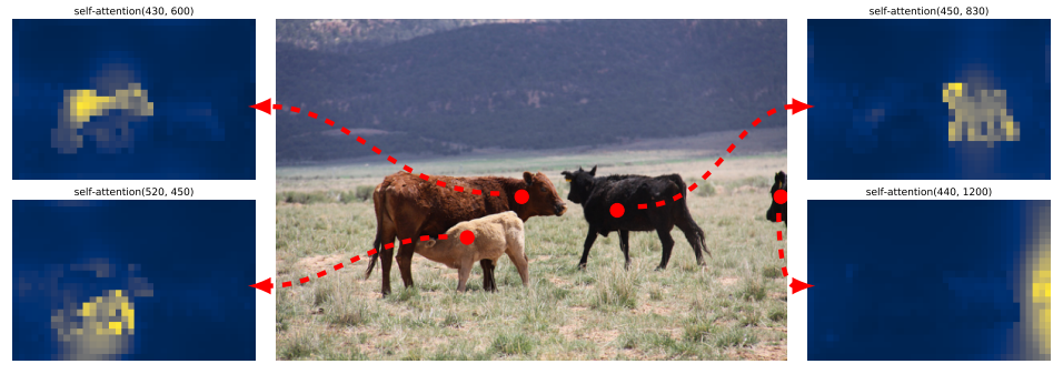
  • Encoder self-attention is able to separate individual instances.
    
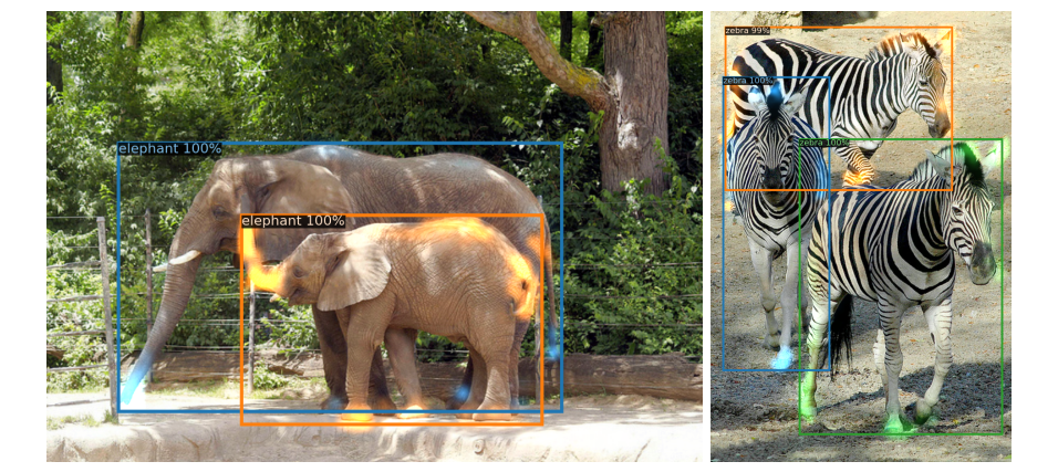
  • Attention socres for every predicted object. Decoder typically attends to object extremities.
    
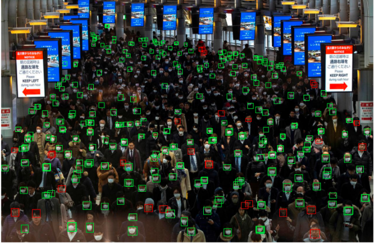
  • Limitations: underperforms on small objects (https://github.com/facebookresearch/detr/issues/216)
    

---

📙 강의

• 이준석 - 시각적 이해를 위한 머신러닝