16. Segmentation

16.1. Semantic Segmentation

16.1.1. Deconvolution Network

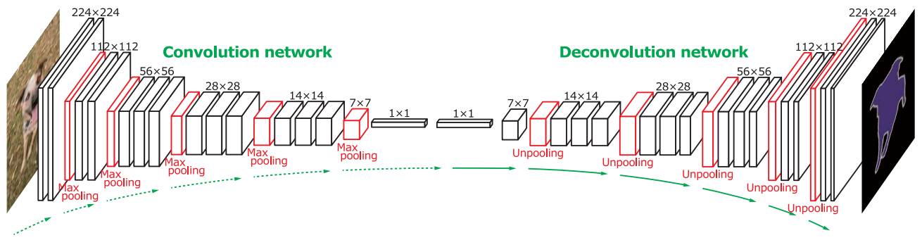
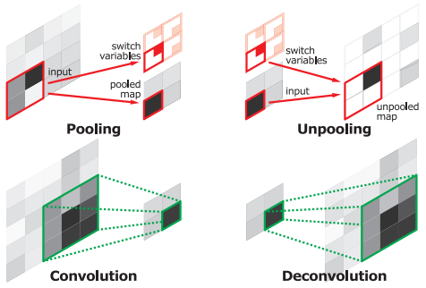
• Unpooling
  • Spatial information within a receptive field is lost during pooling, which may be critical for precise localization that is required for semantic segmentation.
  • To resolve such issue, unpooling layers reconstruct the original size of activations and place each activation back to its original pooled location.
• Deconvolution
  • The output of an unpooling layer is an enlarged, yet sparse activation map.
  • The deconv layers densify the sparse activations obtained by unpooling through conv-like operations with multiple learned filters.

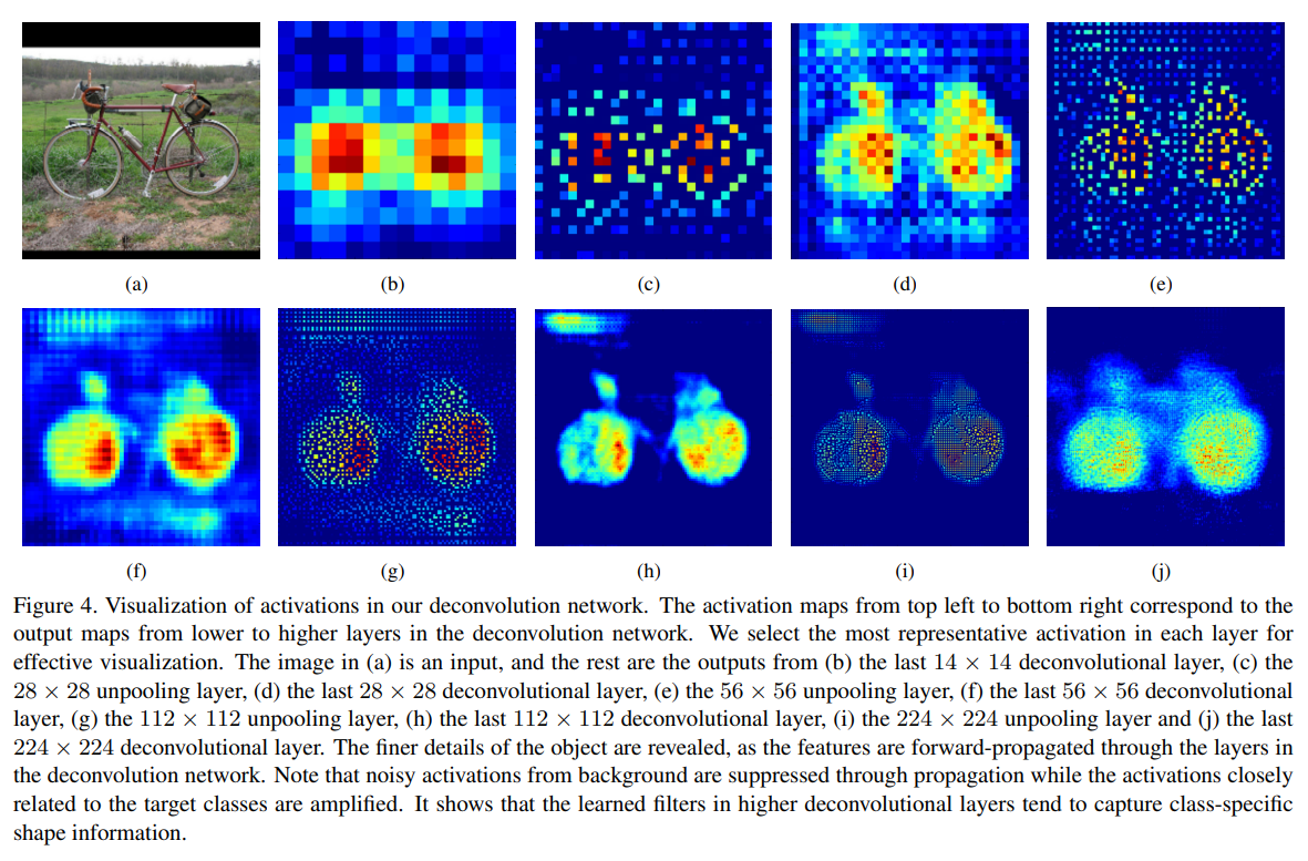
• Analysis of Deconv Net
  • Since unpooling captures example-specific structures by tracing the original locations, it effectively reconstructs the detailed structure of an object in finer resolutions.
  • Learned filters in deconv layers captures class-specific shapes. Through deconv, the activations closely related to the targe classes are amplified while noisy activations from other regions are suppressed effectively.

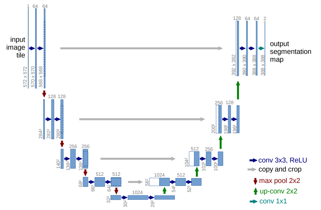
16.1.2. U-Net

• Network Architecture

  • The network consists of a contracting path (left side) and an expansive path (right side).
  • Every step in the expansive path consists of
    • an upsampling of the feature map followed by a $2 \times 2$ convolution ("up-convolution")
    • a concatenation with the correspondingly cropped feature map from the contracting path
    • two $3 \times 3$ conv

• Loss

  $E = \sum_{x \in \Omega} w(\text{x}) \log (p_{l(\text{x})} (\text{x}))$
  • Softmax
    $p_k(\text{x}) = \exp (a_k(\text{x})) / \left (\sum_{k'=1}^K \exp (a_{k'}(\text{x})) \right)$
  • Weight map
    $w(\text{x}) = w_c(\text{x}) + w_0 \cdot \exp \left( - \frac{(d_1(\text{x}) + d_2(\text{x}))^2}{2 \sigma^2} \right)$
    A pixel-wise loss weight force the network to learn the border pixels.
    

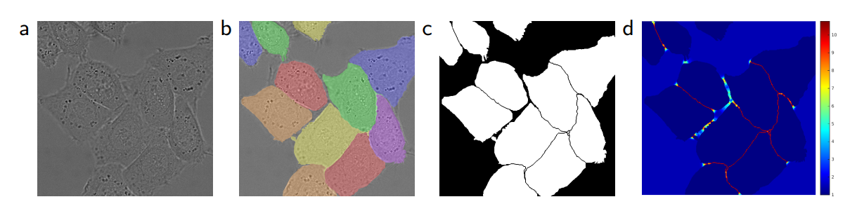
16.2. Instance Segmentation

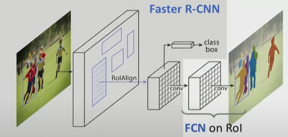
16.2.1. Mask R-CNN

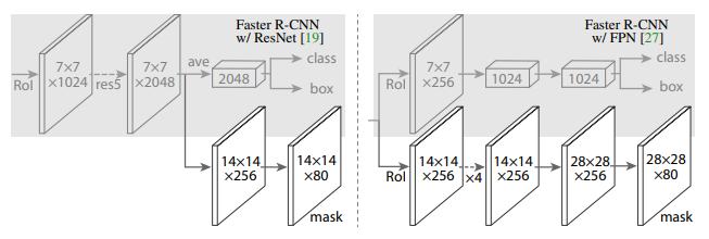
• Network Architecture

  • Faster R-CNN with FCN on RoIs
    • FCN: Fully Convolutional Networks for Semantic Segmentation

• RoIAlign
  

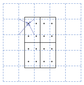
  • RoIPool performs quantization which introduces misalignments between the RoI and the extracted features. While this may not impact classfication, it has a large negative effect on predicting pixel-accurate masks.
  • RoIAlgin removes the harsh quantization of RoIPool, using bilinear interpolation. So, there is no information loss.

16.3. Segmentation with Transformers

16.3.1. Segmenter

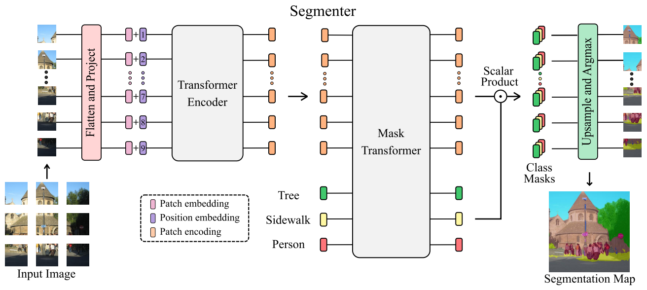
Segmenter is based on a fully transformer-based encoder-decoder architecture mapping a sequence of a patch embeddings to pixel-level class annotations. Its approach relies on a ViT backbone and introduces a mask decoder inspired by DETR.

• Architecture

  • Encoder

    • building upon the ViT (참고: zzwon1212 - ViT)

  • Decoder

    • The sequence of patch encodings $\text{z}_\text{L} \in \mathbb{R}^{N \times D}$ is decoded to a segmentation map: $\text{S} \in \mathbb{R}^{H \times W \times K}$ where $K$ is the number of classes.

    • Flow

      • patch-level encodings coming from the encoder
        ↓ (are mapped by learned decoder)
      • patch-level class scores
        ↓ (are upsampled by bilinear interpolation)
      • pixel-level scores

    • Mask Transformer

      • $\text{L2}$-normalized patch embeddings output by the decoder
        $\text{z}'_\text{M} \in \mathbb{R}^{N \times D}$
      • Class embeddings output by the decoder
        $\text{c} \in \mathbb{R}^{K \times D}$
        The class embeddings are initialized randomly and learned by the decoder.
      • The set of class masks
        $\text{Masks}(\text{z}'_{\text{M}}, \text{c}) = \text{z}'_{\text{M}} \text{c}^T \in \mathbb{R}^{N \times K}$
      • Reshaped 2D mask
        $\text{s}_{\text{mask}} \in \mathbb{R}^{H/P \times W/P \times K}$
      • Bilinearly upsampled feature map
        $\text{s} \in \mathbb{R}^{H \times W \times K}$
      • Final segmentation map is obtained after softmax.

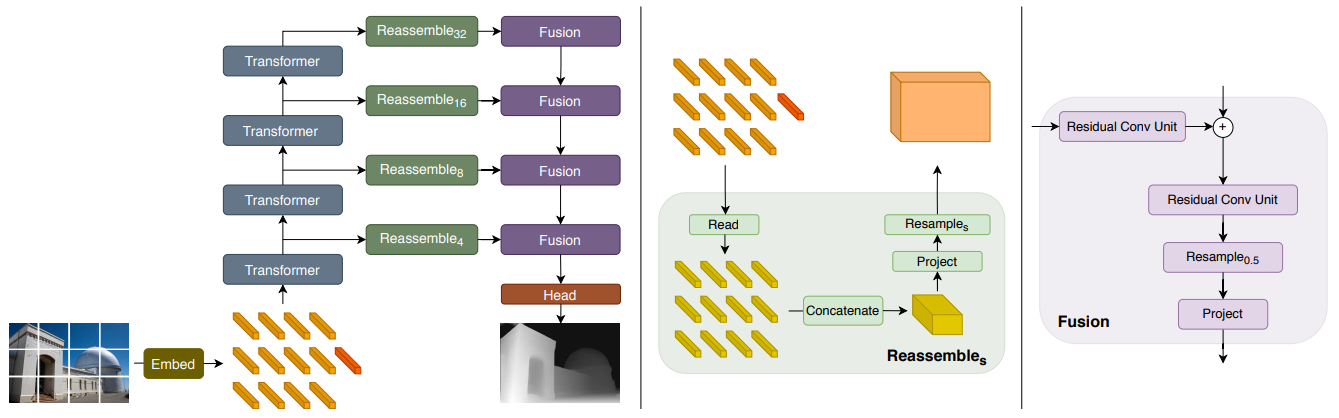
16.3.2. DPT (Dense Prediction Transformer)

• Overview
  Contextualized tokens at specific transformer layers are reassembled by convolution. Then, reassembled feature maps are fed into fusion block which performs convolution. Finally, a task-specific output head is attached to produce the final prediction.

• Receptive field

  • CNNs
    progressively increase their receptive field as feature pass through consecutive layers.
  • Transformer
    has a global receptive filed at every stage after the initial embedding.

• Transformer Encoder

  • DPT use ViT as a backbone architecture.
  • image
    $\mathrm{x} \in \mathbb{R}^{H \times W \times C}$
  • # tokens
    $N_p = \frac{H}{p} \cdot \frac{W}{p}$
    $p$ is the resolution of image patch. ($p = 16$ in the paper)
  • sequence of flattend 2D patches
    $\mathrm{x}_p \in \mathbb{R}^{N_p \times (p^2 \cdot C)}$
  • trainable linear projection
    $\mathbf{E} \in \mathbb{R}^{(p^2 \cdot C) \times D}$
  • patch embedding $t^0$
    $\{\mathrm{x_{class}}, \mathrm{x}_p^1 \mathbf{E},\mathrm{x}_p^2 \mathbf{E}, ..., \mathrm{x}_p^{N_p} \mathbf{E}\} \\ \, \\ t_{n}^0 = \mathrm{x}_p^{n} \mathbf{E}, \,\,\, t_{n}^0 \in \mathbb{R}^D \\ \, \\ t^0 = \{t_0^0, ..., t_{N_p}^0\}, \,\,\, t^0 \in \mathbb{R}^{(N_p + 1) \times D} \\ \, \\$
  • $D = 768$ (for ViT-Base)
    Feature dimensions > # pixels in an input patch
    ↓
    Embedding procedure can learn to retain information if it is beneficial for the task.

• Convolutional Decoder

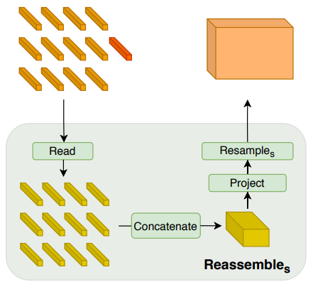
  • Reassemble operation
    
    $\text{Reassemble}_s^{\hat{D}}(t) = (\text{Resample}_s \circ \text{Concatenate} \circ \text{Read}) (t)$
    Features from deeper layers of the transformer are assembled at lower resolution.
    Features from early layers are assembled at higher resolution.
    • Stage 1: Read
      $\mathbb{R}^{(N_p + 1) \times D} \rightarrow \mathbb{R}^{N_p \times D}$
      There are three different variants of this mapping, (ignore, add, proj)
    • Stage 2: Concatenate
      $\mathbb{R}^{N_p \times D} \rightarrow \mathbb{R}^{\frac{H}{p} \times \frac{W}{p} \times D}$
      Reshape $N_p$ tokens into an image-like representation (Recall $N_p = \frac{H}{p} \cdot \frac{W}{p}$)
    • Stage 3: Resample
      $\mathbb{R}^{\frac{H}{p} \times \frac{W}{p} \times D} \rightarrow \mathbb{R}^{\frac{H}{s} \times \frac{W}{s} \times \hat{D}}$
      • Use $1 \times 1$ conv to project the representation to $\hat{D}$ ($\hat{D} = 256)$.
      • Use (strided) $3 \times 3$ conv or transpose conv to implement donwsampling or upsampling.
  • Fusion block
    
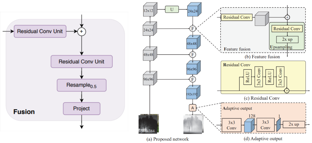
    • Combine the extracted feature maps from consecutive stages using a RefineNet-based feature fusion block.
    • Progressively upsample the representation by a factor of two in each fusion stage. (e.g. $7 \times 7$ → $14 \times 14$ → $28 \times 28$ → $56 \times 56$ → $112 \times 112$)
    • The final representation size has half the resolution of the input image. (e.g. $112 \times 112$ representation for $224 \times 224$ image)
    • Attach a task-specific output head to produce the final prediction.

---

📙 강의

• 이준석 - 시각적 이해를 위한 머신러닝