
실습목표
- 선형회귀 모델을 이용해 주택가격을 예측해보자
# 데이터 전처리 및 탐색용 라이브러리
import numpy as np
import pandas as pd
import matplotlib.pyplot as plt
import seaborn as sns
# 경고창 무시
import warnings
warnings.filterwarnings('ignore')
🔰 머신러닝 프로세스
1. 문제정의
- 호주의 주택가격을 예측하는 모델을 만들어보자
2. 데이터 수집
- kaggle에 오픈된 데이터셋 활용
# 데이터 읽어오기
house_data = pd.read_csv('data/melb_data.csv')
house_data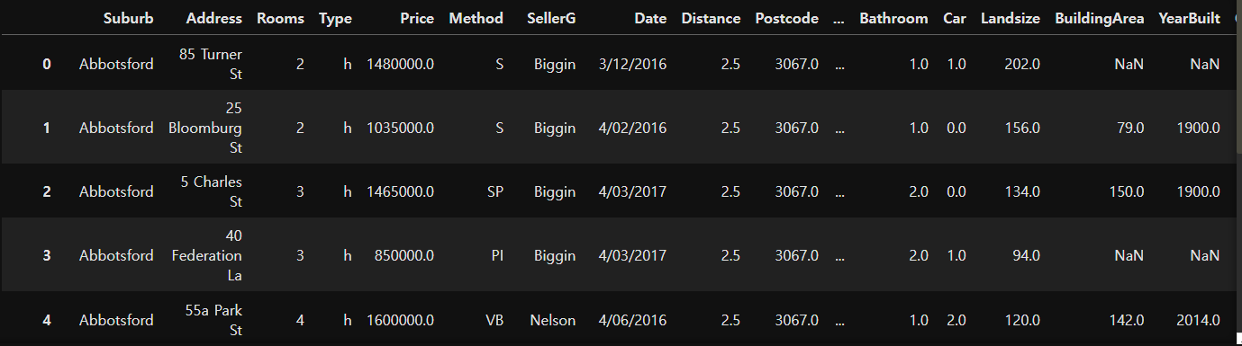
# 데이터 정보 확인
# 입력특성과 정답특성을 확인
# 20개의 모든 입력특성을 사용하는 게 좋다 ? -> 관련이 있는 특성을 골라 활용하는 게 좋다(특성선택)
# 결측치가 있는 컬럼 파악 -> 결측치가 있으면 분석/학습에 활용하기 어렵다 -> 전처리 필요
# 데이터 타입 화인 -> object로 되어있는 타입은 문자일 가능성이 높다 -> 숫자 형태로 변환 필요
house_data.info()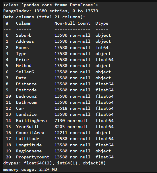
# 기술통계량
# house_data.describe() # 수치형 기술통계량 확인 가능
# house_data.describe(include='all') # 수치형, 범주형 모두 기술통계량 확인 가능
house_data.describe(include='object') # 원하는 데이터 타입만 필터링해서 확인 가능 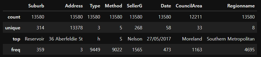
# Rooms : 방의 개수에 따른 주택가격의 분포현황 확인
plt.figure(figsize=(10,4))
sns.boxplot(data=house_data, # 활용할 데이터
           x="Rooms", y="Price")
plt.show()
# 방 개수가 증가할수록 주택가격의 중앙값이 상승
# 하지만 5개 이상은 변하는 폭이 적다 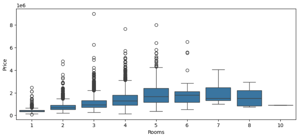
# 방의 개수가 3개인 데이터 추출 후 통계치 확인
house_data[house_data['Rooms']==3].describe()

# 4분위 수 값을 이용해서 이상치 삭제도 가능! 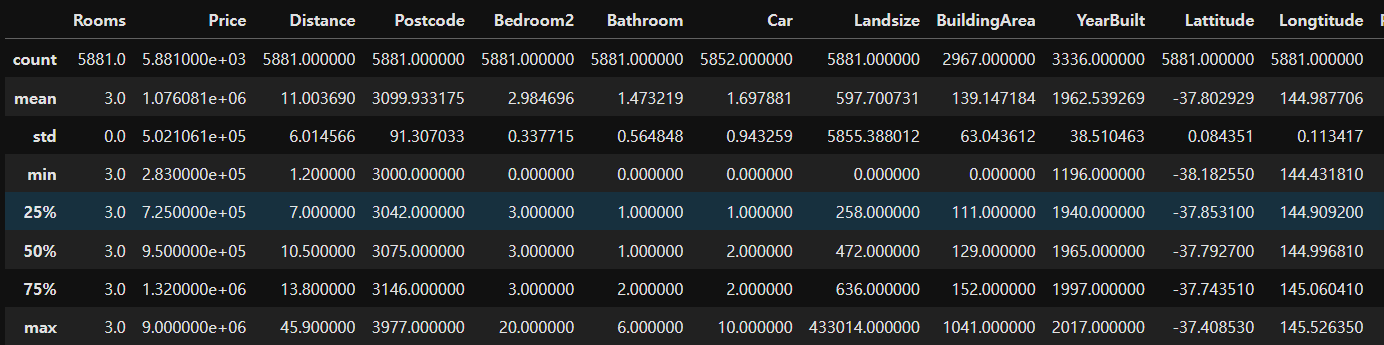
# 주택타입 종류 확인
house_data['Type'].unique() 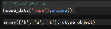
house_data[['Type','Price']].groupby(by='Type').mean()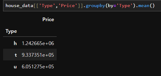
# 한글폰트 설정하기
plt.rc('font',family="Malgun Gothic")
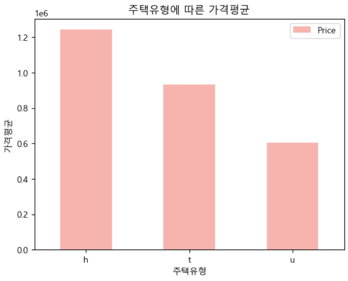
# 주택타입에 따른 가격평균 bar chart 시각화
house_data[['Type','Price']].groupby(by='Type').mean().plot(kind='bar', colormap='Pastel1', rot=0,
xlabel="주택유형",ylabel="가격평균",
title="주택유형에 따른 가격평균")
# 주택에 따라서 가격의 평균차이가 있다 -> 타입이 가격에 영향을 준다
# 위도와 가격의 KDE(밀도추정) 그래프 시각화
plt.figure(figsize=(10,5))
sns.kdeplot(data=house_data, x="Lattitude", y="Price",
           fill=True)
plt.show()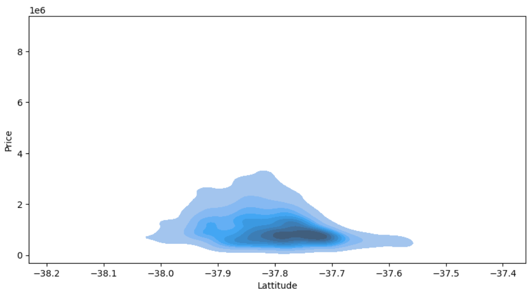
# 경도와 가격의 KDE(밀도추정) 그래프 시각화
plt.figure(figsize=(10,5))
sns.kdeplot(data=house_data, x="Longtitude", y="Price",
           fill=True)
plt.show()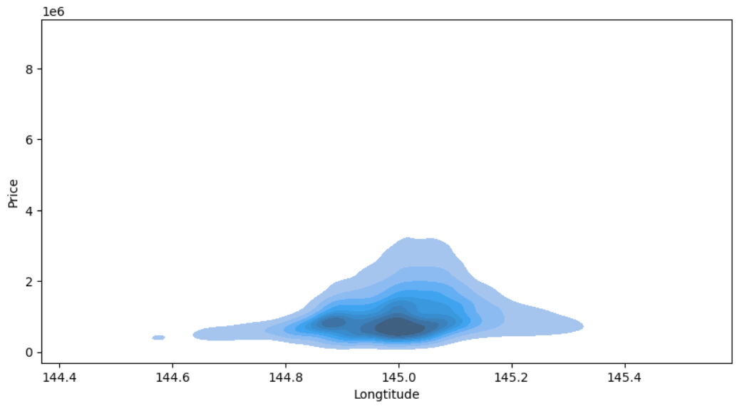
# 위도와 경도 시각화
plt.figure(figsize=(10,5))
sns.kdeplot(data=house_data, x="Lattitude", y="Longtitude",
           fill=True)
plt.show()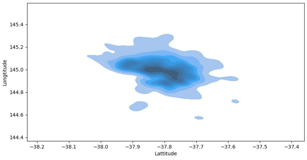
3. 데이터 전처리 및 탐색
결측치 처리하기
- 결측치가 있는 데이터를 삭제하거나 결측치를 대체값으로 채우는 선택을 할 수 있다.
- 데이터 양이 많은 경우 결측치를 삭제해도 무방하나 데이터 양이 적다면 대체값을 채우는 게 좋은 선택이 될 수 있다. 단, 대체값의 경우 올바른 값이 아니면 분석을 방해할 가능성이 있다.
# 결측치가 있는 특성 확인  # True값이 1로 count
house_data.isnull().sum().sort_values(ascending=False)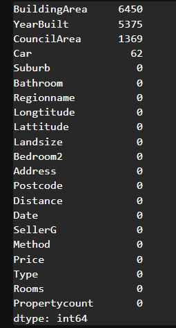
house_data.isnull().sum().sort_values(ascending=False)/len(house_data)*100
# 결측치 비율이 높은 컬럼들은 활용할 때 신중히 고민해야 한다 -> 대체값 채울 때도 정교하게 진행해야 함
# 결측치 비율이 상대적으로 낮은 CouncilArea와 Car를 전처리해보자
# 기술통계를 확인하여 결측치 채우기
house_data['Car'].describe()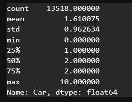
# 결측치를 채우는 함수 -> filna
house_data['Car'] = house_data['Car'].fillna(0)
# Suburb(지역이름)을 통해서 CouncilArea(관할구역) 결측치를 채워보자
house_data.pivot_table(index=['Suburb','CouncilArea'], # 행에 표현될 컬럼선택
values='Rooms', # 결측치 없는 컬럼 선택
aggfunc='count') # 갯수를 세어주는 집계함수 설정 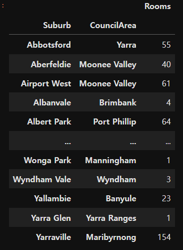
# 최빈값으로 구성된 테이블 생성
council_mode_table = house_data.groupby('Suburb')['CouncilArea'].agg(pd.Series.mode)
council_mode_table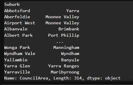
# apply 함수를 이용해서 각 행마다 결측치를 처리
def fill_council(row):
    display(row)
# apply 함수를 이용해서 각 행마다 결측치를 처리
def fill_council(row):
if pd.isnull(row['CouncilArea']): # 결측치인 경우
return council_mode_table[row['Suburb']]
else:
return row['CouncilArea']house_data['CouncilArea'] = house_data.apply(fill_council, axis=1)# 결측치 비율 확인
house_data.isnull().sum().sort_values(ascending=False)/len(house_data)*100 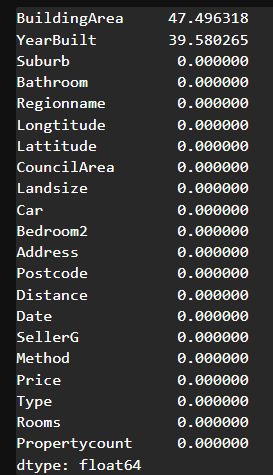
# 각 컬럼과 Price 사이의 상관계수(correlation) 확인
house_data.corr(numeric_only=True)['Price'].sort_values()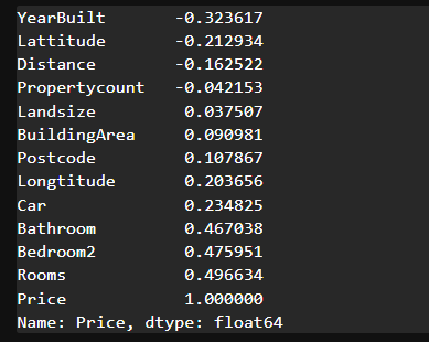
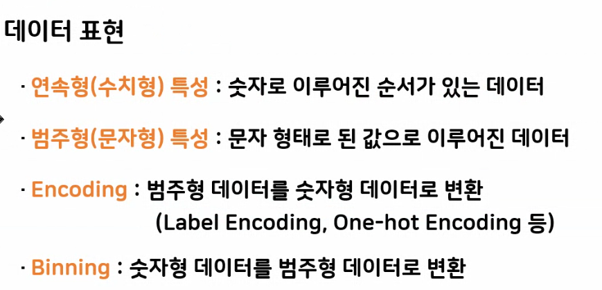
학습을 위한 전처리
- 특성선택
- 글자 -> 숫자 변경(인코딩)
- 지도학습을 위한 문제, 답 분리
- 훈련, 평가 데이터 분리
# 학습에 사용할 입력특성 선택
feature_names = ["Rooms","Bedroom2","Bathroom","Lattitude","Longtitude","Type_encoding","CouncilArea"]
💙인코딩 방법
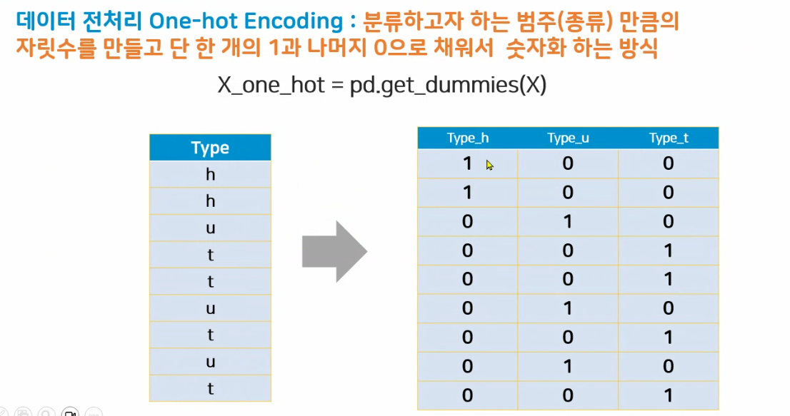
(1) 원핫인코딩
원핫인코딩을 쓰는 경우 : 해당 컬럼에 순서라는 의미가 없는 경우
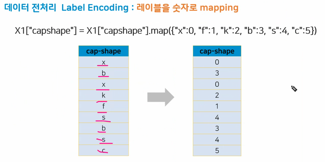
(2) 레이블인코딩
레이블인코딩을 쓰는 경우 : 해당 컬럼에 순서가 부여된 경우
# type은 평균가격이 순서가 있기 때문에 레이블 인코딩을 써볼 수 있겠다.
house_data["Type_encoding"] = house_data['Type'].map({"h":0, "t":1, "u":2})house_data['CouncilArea'].astype('str').unique()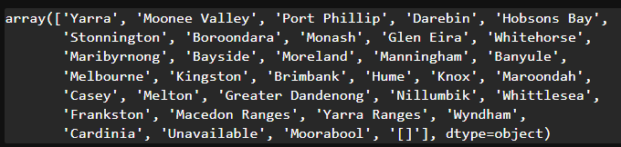
# '[]'가 들어있는 데이터의 index 추출
drop_index = house_data[house_data['CouncilArea']=='[]'].index
drop_index

# drop_index 삭제해주기
house_data.drop(drop_index, inplace=True)
# CouncilArea는 원핫인코딩을 이용해서 동등한 크기를 지니는 숫자로 인코딩
council_one_hot = pd.get_dummies(house_data['CouncilArea'])
council_one_hot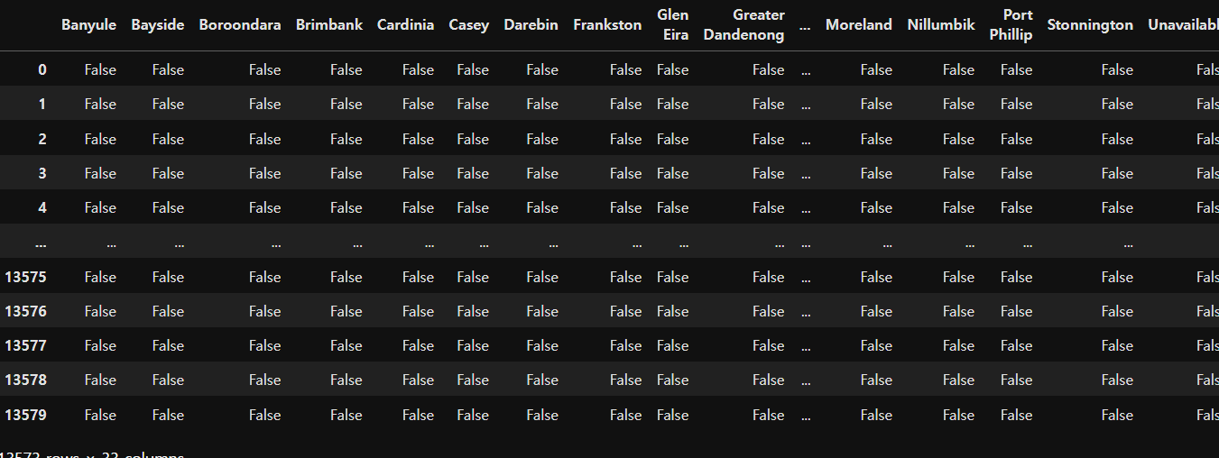
# prefix 사용하여 접두어 넣기
council_one_hot = pd.get_dummies(house_data['CouncilArea'], dtype="int64", prefix="council")
council_one_hot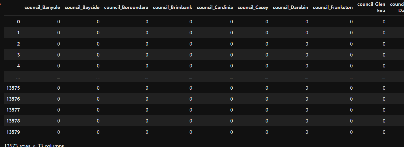
# 선택한 특성 및 인코딩 특성을 병합
df1 = house_data[feature_names]
df1.head()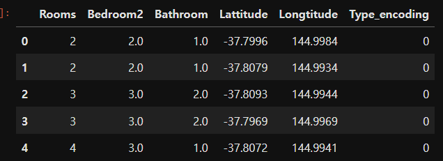
# 문제 (입력특성)
X = pd.concat([df1, council_one_hot], axis=1)
X.head()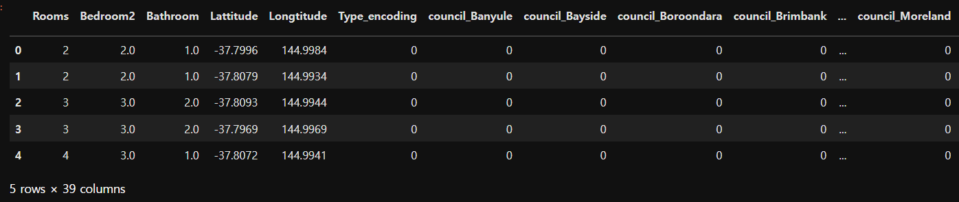
# 정답
y = house_data['Price']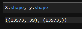
- 훈련용, 평가용으로 분리
- 학습된 모델의 신뢰도를 확보하기 위해 평가용 데이터를 분리
- 보통 7:3의 비율로 분할
- 가능하다면 평가용 데이터가 여러 세트로 확보되면 좋다
from sklearn.model_selection import train_test_split

# train_test_split(문제, 정답, 분리비율, 고정키) # 고정키 -> 데이터를 골고루 섞기 위해 넣음, 신뢰성을 높이기 위해 사용
X_train, X_test, y_train, y_test = train_test_split(X, y, test_size=0.3, random_state=15)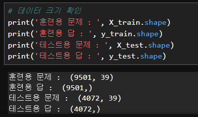
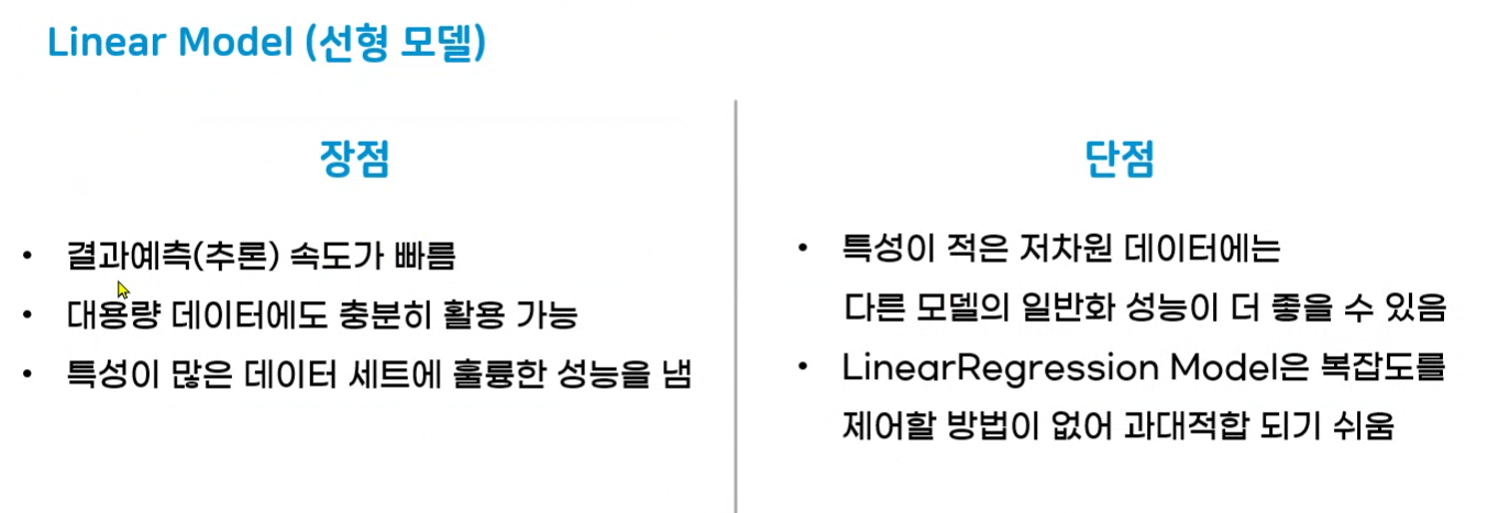
4. 모델 선택 및 학습
# 모델생성
from sklearn.linear_model import LinearRegression
house_model_linear = LinearRegression()
# 모델학습
house_model_linear.fit(X_train, y_train)# 가중치, 절편 확인
# y = wx+b
print('가중치 :', house_model_linear.coef_)
print('절편 :', house_model_linear.intercept_)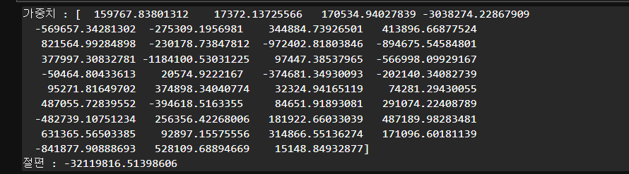
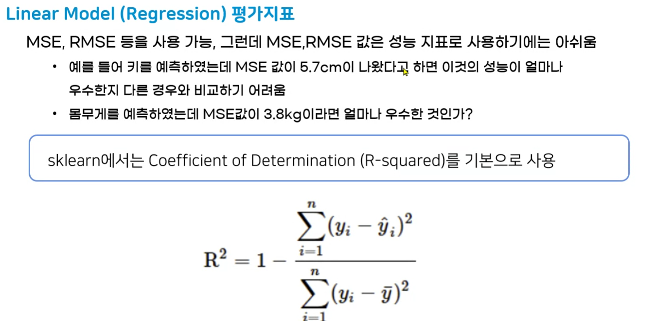
5. 모델평가
# 모델 평가
# score로 점수 내주기
print('Linear Score :', house_model_linear.score(X_test, y_test))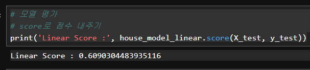
# MSE 구하는 모듈 가져옴
# sklearn.metrics : 평가지표 모음
from sklearn.metrics import mean_squared_error
# 평가지표
linear_pre_test = house_model_linear.predict(X_test)
print('MSE :', mean_squared_error(y_test, linear_pre_test)) # 실제값과 예측값의 차이
print('RMSE :', mean_squared_error(y_test, linear_pre_test)**0.5) # 평균제곱오차제곱근
# 제곱값은 실제 오차에 제곱이 되므로 실제를 알아보기 힘듦
# 실제 단위 달러 제곱근 씌워주기
# 40만 달러의 차이 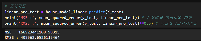
6. 모델활용
- 추후 서비스 제작시 사용

Hello, World!