
[실습] unsmile 데이터 토큰화 및 수치화 : BOW
# countvectorizer를 이용하기 위해서 문장을 하나로 합쳐주는 작업이 필요
clean_morphs_train2 = [ " ".join(s) for s in clean_morphs_train]
clean_morphs_test2 = [ " ".join(s) for s in clean_morphs_test]
clean_morphs_test2[:4]
unsmile_cv = CountVectorizer(stop_words=['이다', '으로', '하고', '부터'],
ngram_range=(1,2), # n-gram 설정 (유비~바이
# 한단어 토큰(1,1) 대표값
# ngram_range[2,2] 두 단어를 묶는게 도움이 되겠다.
max_df = 0.9, # 최대 등장빈도
min_df = 8) # 최소 등장빈도
unsmile_cv.fit(clean_morphs_train2) # 단어사전 구축
# 오타.. 등으로 회수가 적음 불필요한 단어 토큰일 가능성 높음
# CountVectorizer할 때 옵션을 줄 수 있음
# max_df : 문장에서 최대로 등장할 수 있는 횟수 지정
# 전체데이터에서 과하게 많이 나오는 단어들을 제어할 수 있다. 카운트 최대횟수
# min_df : 전체 댓글에서 한번 나오는 댓글 -> 분석에 중요하지 않다. 성능에 민감하게 적용. len(unsmile_cv.vocabulary_) # 단어사전의 크기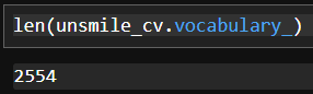
unsmile_cv.vocabulary_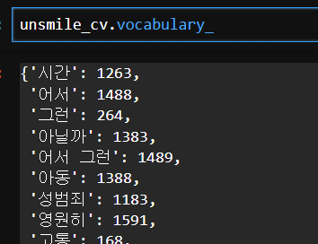
# 훈련용과 평가용 데이터 수치화
train_transformed_BOW = unsmile_cv.transform(clean_morphs_train2)
test_transformed_BOW = unsmile_cv.transform(clean_morphs_test2)train_transformed_BOW, test_transformed_BOW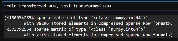
선형분류모델 학습 및 평가
# 정답데이터 추출
y_train = train.loc[:,"여성/가족":"clean"].values.argmax(axis=1)
y_test = test.loc[:,"여성/가족":"clean"].values.argmax(axis=1)y_train.shape, y_test.shape 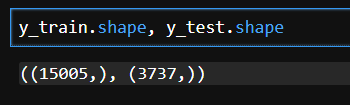
from sklearn.linear_model import LogisticRegression
from sklearn.model_selection import cross_val_score
# 로지스틱 모델 생성
unsmile_logi = LogisticRegression(max_iter=1000)
# 교차검증
score_BOW = cross_val_score(unsmile_logi, train_transformed_BOW, y_train, cv=5) score_BOW.mean() 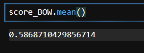
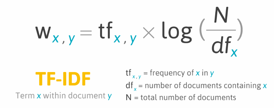
💠 TF-IDF
- 말뭉치(corpus) : 텍스트마이닝,자연어처리 분야에서 학습을 위해 사용하는 데이터셋
- 문서(document) : 말뭉치에서 각 샘플을 치징하는 단어
- TF(Term Frequency) : 하나의 문서(document)에서 개별 단어들이 등장하는 빈도 수
- DF(Document Frequency) : 하나의 단어(토큰)가 전체 말뭉치에서 등장하는 문서(document) 수
# TF-IDF : 하나의 문서에서는 자주 등장하고 전체 문서에서는 적당히 등장하는 단어의 가치를 측정
from sklearn.feature_extraction.text import TfidfVectorizer
# step 1 : 단어사전 구축
sample_tf_idf = TfidfVectorizer()
sample_tf_idf.fit(sample_text2)# step 2 : 수치화
sample_tf_idf.transform(sample_text2).toarray()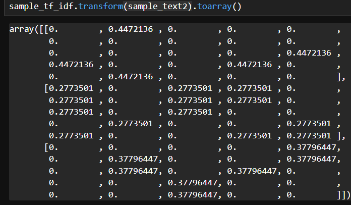
[실습] unsmile 데이터셋 토큰화 및 수치화 : TF-IDF
# 1. TF-IDF를 이용해 혐오표현 데이터 토큰화 및 수치화
unsmile_cv_tfidf = TfidfVectorizer(stop_words=['이다', '으로', '하고', '부터'],
                             ngram_range=(1,2), # n-gram 설정 (유비~바이)
                             max_df = 0.9, # 최대 등장빈도
                             min_df = 8) # 최소 등장빈도
unsmile_cv_tfidf.fit(clean_morphs_train2) # 단어사전 구축
# 훈련용과 평가용 데이터 수치화
train_transformed_tfidf = unsmile_cv_tfidf.transform(clean_morphs_train2)
test_transformed_tfidf = unsmile_cv_tfidf.transform(clean_morphs_test2)train_transformed_tfidf, test_transformed_tfidf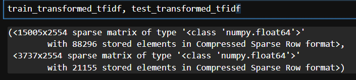
모델링
# 2. 선형분류모델 객체 생성
unsmile_logi_for_tfidf = LogisticRegression(max_iter=1000)
# 3. 교차검증 실시
score_tfidf = cross_val_score(unsmile_logi_for_tfidf, train_transformed_tfidf, y_train, cv=5)
score_tfidf.mean()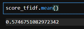
하이퍼파라미터 튜닝 with GridSearch
- LogisticRegression : C(규제)
- TfidfVectorizer : ngram_range, max_df, min_df
# if-idf와 logistic 두 개를 튜닝해보자
# 하나의 파이프라인으로 묵어서 튜닝
from sklearn.pipeline import Pipeline # 파이프라인 구축 클래스
from sklearn.model_selection import GridSearchCV # 하이퍼파라미터튜닝을 도와주는 클래스 # CV: Cross Validation
# 파이프라인 생성
unsmile_pipline = Pipeline([
('unsmile_tf_idf', TfidfVectorizer()),
('unsmile_logi', LogisticRegression())
])# 튜닝할 파라미터 셋팅
grid_prams = {
"unsmile_logi__C" : [0.001, 0.01, 0.1, 1, 10, 100, 1000], # 규제가 강한 것부터 약한 것까지
"unsmile_tf_idf__max_df" : [0.7, 0.8, 0.9], # 최대등장 빈도
"unsmile_tf_idf__min_df" : [5, 8, 10, 15], # 최소등장 빈도
"unsmile_tf_idf__ngram_range" : [(1,1), (1,2), (1,3)] # n-gram
}grid = GridSearchCV(unsmile_pipline, # 튜닝할 모델
grid_prams, # 튜닝할 파라미터
cv = 3, # 조합당 실행할 교차검증 횟수
n_jobs = -1) # PC자원을 연산에 집중시키는 파라미터 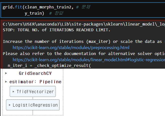
# best score
grid.best_score_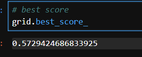
# best param 조합
grid.best_params_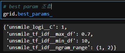
# best model
best_model = grid.best_estimator_
# 베스트모델 저장
with open("./best_unsmiled_model.pkle", "wb") as f :
pickle.dump(best_model, f)테스트데이터 활용 평가 및 시각화
# 분류평가지표 리포팅(쩡확도, 재현율, 정밀도, f1-score 확인 가능)
from sklearn.metrics import classification_reporttrain.columns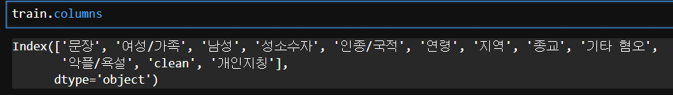
y_pre = best_model.predict(clean_morphs_test2)
print(classification_report(y_test, y_pre)) # 실제정답, 예측값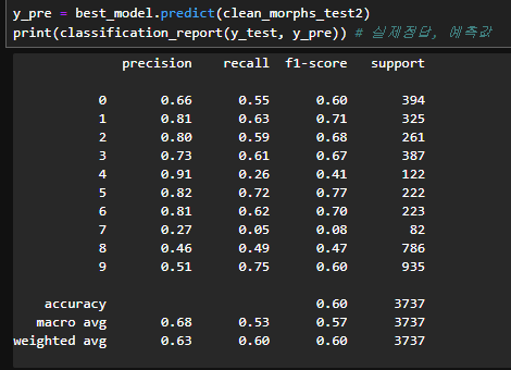
f1-score가 가장 높음
# 베스트 모델 로딩
with open("./best_unsmiled_model.pkl","rb") as f:
    best_model = pickle.load(f)
# 사용하는 단어사전 추출, 각 단어의 가중치 추출
unsmile_vocab = best_model.steps[0][1].vocabulary_
unsmile_weighs = best_model.steps[1][1].coef_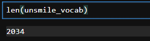
# 각 클래스별로 단어의 가중치를 가지고 있다
# 학습결과가 그나마 제일 좋은 5번(지역혐오) 가중치를 활용해서 시각화 해보자
unsmile_weighs.shape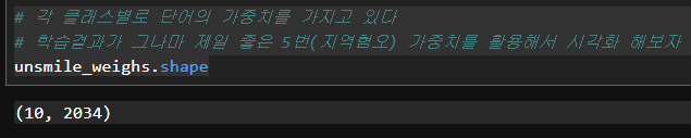
# vocab의 단어를 순서대로 정렬한 후 가중치를 결합해서 df로 만들자
# 가중치 - 지역혐오 [5] 얼마나 중요한 영향을 주는지 확인
# 인덱스 컬럼을 인덱스로 이동
# 가중치 정렬 양수 - 지역혐오가 높다라고 학습, 상위30개
import pandas as pd
unsmile_df = pd.DataFrame([unsmile_vocab.keys(),unsmile_vocab.values()]).T
unsmile_df.columns = ['단어','인덱스']
unsmile_df.sort_values(by='인덱스', inplace=True)
unsmile_df['가중치'] = unsmile_weighs[5]
unsmile_df.set_index('인덱스',inplace=True)
hate_top_30 = unsmile_df.sort_values(by='가중치',ascending=False).head(30)
hate_top_30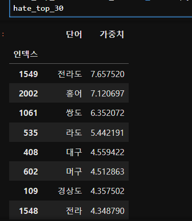
# pie chart 로 시각화
import matplotlib.pyplot as plt
plt.rc('font',family = 'Malgun Gothic')
hate_top_30.set_index('단어').plot(kind='pie', subplots=True,
                                 figsize=(20,20),startangle=90,
                                 counterclock=False, autopct='%.1f%%')
# squarity 시각화
! pip install squarifyimport squarify
import matplotlibplt.figure(figsize=(15,15)) # 가로, 세로 크기 설정
sizes = hate_top_30['가중치']
labels = hate_top_30['단어']
# 빈도값을 0~1까지 값을 갖도록 min-max 표준화
norm = matplotlib.colors.Normalize(vmin=min(sizes),
vmax=max(sizes))
# 정규화된 값을 matplotlib의 cm(color map)에서 Blue 에 적용
colors = [matplotlib.cm.Reds(norm(value)) for value in sizes]
squarify.plot(sizes, 10, 10, label=labels, color=colors,
bar_kwargs=dict(linewidth=8, edgecolor="#eee"),
text_kwargs=dict(fontsize=25))
plt.title('혐오에 활용되는 주요 키워드', fontdict=dict(fontsize=25))
plt.axis('off') # x,y축 off
plt.show() # 그림 출력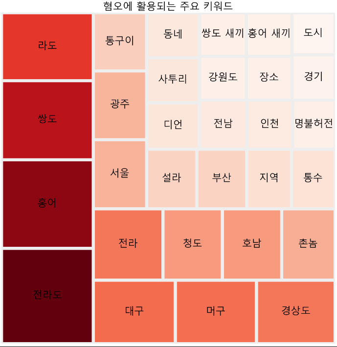

Hello, World!