Computer vision - Section 1

Object Detection - 두 개 이상의 Object를 검출

그림에서 detect하려는 object가 어디에 위치해 있는지를 찾는것이 목표.

Sliding Window 방식

Window를 왼쪽 상단에서부터 오른쪽 하단으로 이동시키면서 Object를 Detection하는 방식

• Object Detection의 초기 기법으로 활용
• Object가 없는 영역도 무조건 슬라이딩 해야하고, 여러 형태의 window와 여러 scale을 가진 이미지를 스캔해서 검출해야 하므로 수행시간이 오래걸리고 검출 성능이 상대적으로 낮음
• Region Proposal(영역 추정) 기법의 등장으로 활용도는 떨어졌지만 Object Detection 발전을 위한 기술적 토대를 제공함

Region Proposal (영역 추정) 방식

Object가 있을 만한 후보 영역을 찾는 것

Selective Search - Region Proposal의 대표 방법

• 빠른 Detection과 높은 Recall 예측 성능을 동시에 만족하는 알고리즘
• 컬러, 무늬(Texture), 크기(Size), 형태(Shape)에 따라 유사한 Region을 계층적 그루핑 방법으로 계산
• Selective Search는 최초에는 Pixel Intensity기반한 graph-based segment 기법에 따라 Over Segmentation을 수행

Selective Search의 수행 프로세스

1. 개별 Segment된 모든 부분들을 Bounding box로 만들어서 Region Proposal 리스트로 추가
2. 컬러, 무늬(Texture), 크기(Size), 형태(Shape)에 따라 유사도가 비슷한 Segment들을 그룹핑함
3. 다시 1번 Step Region Proposal 리스트 추가, 2번 Step 유사도가 비슷한 Segment들 그룹핑을 계속 반복 하면서 Region Proposal을 수행

Selective Search 실습 및 시각화

selectivesearch를 설치하고 이미지를 로드

!pip install selectivesearch

import selectivesearch
import cv2
import matplotlib.pyplot as plt
import os
%matplotlib inline

### 오드리헵번 이미지를 cv2로 로드하고 matplotlib으로 시각화 
img = cv2.imread('./data/audrey01.jpg')
img_rgb = cv2.cvtColor(img, cv2.COLOR_BGR2RGB)
print('img shape:', img.shape)

plt.figure(figsize=(8, 8))
plt.imshow(img_rgb)
plt.show()

import selectivesearch 

#selectivesearch.selective_search()는 이미지의 Region Proposal정보를 반환 
_, regions = selectivesearch.selective_search(img_rgb, scale=100, min_size=2000)

print(type(regions), len(regions))

"""
<class 'list'> 41
"""

41개의 regions가 있는 것을 확인

반환된 Region Proposal(후보 영역)에 대한 정보 보기.

반환된 regions 변수는 리스트 타입으로 세부 원소로 딕셔너리를 가지고 있음. 개별 딕셔너리내 KEY값별 의미

• rect 키값은 x,y 시작 좌표와 너비, 높이 값을 가지며 이 값이 Detected Object 후보를 나타내는 Bounding box임.
• size는 segment로 select된 Object의 크기
• labels는 해당 rect로 지정된 Bounding Box내에 있는 오브젝트들의 고유 ID
• 아래로 내려갈 수록 너비와 높이 값이 큰 Bounding box이며 하나의 Bounding box에 여러개의 오브젝트가 있을 확률이 커짐.

regions

"""
[{'labels': [0.0], 'rect': (0, 0, 107, 167), 'size': 11166},
 {'labels': [1.0], 'rect': (15, 0, 129, 110), 'size': 8771},
 {'labels': [2.0], 'rect': (121, 0, 253, 133), 'size': 17442},
 {'labels': [3.0], 'rect': (134, 17, 73, 62), 'size': 2713},
 {'labels': [4.0], 'rect': (166, 23, 87, 176), 'size': 8639},
 {'labels': [5.0], 'rect': (136, 53, 88, 121), 'size': 4617},
 {'labels': [6.0], 'rect': (232, 79, 117, 147), 'size': 7701},
 {'labels': [7.0], 'rect': (50, 91, 133, 123), 'size': 7042},
 {'labels': [8.0], 'rect': (305, 97, 69, 283), 'size': 11373},
 {'labels': [9.0], 'rect': (0, 161, 70, 46), 'size': 2363},
 {'labels': [10.0], 'rect': (72, 171, 252, 222), 'size': 34467},
 {'labels': [11.0], 'rect': (0, 181, 118, 85), 'size': 5270},
 {'labels': [12.0], 'rect': (106, 210, 89, 101), 'size': 2868},
 {'labels': [13.0], 'rect': (302, 228, 66, 96), 'size': 2531},
 {'labels': [14.0], 'rect': (0, 253, 92, 134), 'size': 7207},
 {'labels': [15.0], 'rect': (153, 270, 173, 179), 'size': 10360},
 {'labels': [16.0], 'rect': (0, 305, 47, 139), 'size': 4994},
 {'labels': [17.0], 'rect': (104, 312, 80, 71), 'size': 3595},
 {'labels': [18.0], 'rect': (84, 360, 91, 67), 'size': 2762},
 {'labels': [19.0], 'rect': (0, 362, 171, 87), 'size': 7705},
 {'labels': [20.0], 'rect': (297, 364, 77, 85), 'size': 5164},
 {'labels': [7.0, 11.0], 'rect': (0, 91, 183, 175), 'size': 12312},
 {'labels': [4.0, 5.0], 'rect': (136, 23, 117, 176), 'size': 13256},
 {'labels': [10.0, 15.0], 'rect': (72, 171, 254, 278), 'size': 44827},
 {'labels': [4.0, 5.0, 3.0], 'rect': (134, 17, 119, 182), 'size': 15969},
 {'labels': [8.0, 13.0], 'rect': (302, 97, 72, 283), 'size': 13904},
 {'labels': [2.0, 6.0], 'rect': (121, 0, 253, 226), 'size': 25143},
 {'labels': [7.0, 11.0, 9.0], 'rect': (0, 91, 183, 175), 'size': 14675},
 {'labels': [0.0, 1.0], 'rect': (0, 0, 144, 167), 'size': 19937},
 {'labels': [0.0, 1.0, 4.0, 5.0, 3.0],
  'rect': (0, 0, 253, 199),
  'size': 35906},
 {'labels': [14.0, 16.0], 'rect': (0, 253, 92, 191), 'size': 12201},
 {'labels': [14.0, 16.0, 7.0, 11.0, 9.0],
  'rect': (0, 91, 183, 353),
  'size': 26876},
 {'labels': [10.0, 15.0, 19.0], 'rect': (0, 171, 326, 278), 'size': 52532},
 {'labels': [10.0, 15.0, 19.0, 8.0, 13.0],
  'rect': (0, 97, 374, 352),
  'size': 66436},
 {'labels': [17.0, 18.0], 'rect': (84, 312, 100, 115), 'size': 6357},
 {'labels': [17.0, 18.0, 14.0, 16.0, 7.0, 11.0, 9.0],
  'rect': (0, 91, 184, 353),
  'size': 33233},
 {'labels': [17.0, 18.0, 14.0, 16.0, 7.0, 11.0, 9.0, 12.0],
  'rect': (0, 91, 195, 353),
  'size': 36101},
 {'labels': [17.0, 18.0, 14.0, 16.0, 7.0, 11.0, 9.0, 12.0, 2.0, 6.0],
  'rect': (0, 0, 374, 444),
  'size': 61244},
 {'labels': [17.0,
   18.0,
   14.0,
   16.0,
   7.0,
   11.0,
   9.0,
   12.0,
   2.0,
   6.0,
   10.0,
   15.0,
   19.0,
   8.0,
   13.0],
  'rect': (0, 0, 374, 449),
  'size': 127680},
 {'labels': [17.0,
   18.0,
   14.0,
   16.0,
   7.0,
   11.0,
   9.0,
   12.0,
   2.0,
   6.0,
   10.0,
   15.0,
   19.0,
   8.0,
   13.0,
   20.0],
  'rect': (0, 0, 374, 449),
  'size': 132844},
 {'labels': [17.0,
   18.0,
   14.0,
   16.0,
   7.0,
   11.0,
   9.0,
   12.0,
   2.0,
   6.0,
   10.0,
   15.0,
   19.0,
   8.0,
   13.0,
   20.0,
   0.0,
   1.0,
   4.0,
   5.0,
   3.0],
  'rect': (0, 0, 374, 449),
  'size': 168750}]
"""

# rect정보만 출력해서 보기
cand_rects = [cand['rect'] for cand in regions]
print(cand_rects)

"""
[(0, 0, 107, 167), (15, 0, 129, 110), (121, 0, 253, 133), (134, 17, 73, 62), (166, 23, 87, 176), (136, 53, 88, 121), (232, 79, 117, 147), (50, 91, 133, 123), (305, 97, 69, 283), (0, 161, 70, 46), (72, 171, 252, 222), (0, 181, 118, 85), (106, 210, 89, 101), (302, 228, 66, 96), (0, 253, 92, 134), (153, 270, 173, 179), (0, 305, 47, 139), (104, 312, 80, 71), (84, 360, 91, 67), (0, 362, 171, 87), (297, 364, 77, 85), (0, 91, 183, 175), (136, 23, 117, 176), (72, 171, 254, 278), (134, 17, 119, 182), (302, 97, 72, 283), (121, 0, 253, 226), (0, 91, 183, 175), (0, 0, 144, 167), (0, 0, 253, 199), (0, 253, 92, 191), (0, 91, 183, 353), (0, 171, 326, 278), (0, 97, 374, 352), (84, 312, 100, 115), (0, 91, 184, 353), (0, 91, 195, 353), (0, 0, 374, 444), (0, 0, 374, 449), (0, 0, 374, 449), (0, 0, 374, 449)]
"""

bounding box를 시각화 하기

# opencv의 rectangle()을 이용하여 시각화
# rectangle()은 이미지와 좌상단 좌표, 우하단 좌표, box컬러색, 두께등을 인자로 입력하면 원본 이미지에 box를 그려줌. 

green_rgb = (125, 255, 51)
img_rgb_copy = img_rgb.copy()
for rect in cand_rects:
    
    left = rect[0]
    top = rect[1]
    # rect[2], rect[3]은 너비와 높이이므로 우하단 좌표를 구하기 위해 좌상단 좌표에 각각을 더함. 
    right = left + rect[2]
    bottom = top + rect[3]
    
    img_rgb_copy = cv2.rectangle(img_rgb_copy, (left, top), (right, bottom), color=green_rgb, thickness=2)
    
plt.figure(figsize=(8, 8))
plt.imshow(img_rgb_copy)
plt.show()

bounding box의 크기가 큰 후보만 추출

cand_rects = [cand['rect'] for cand in regions if cand['size'] > 10000]

green_rgb = (125, 255, 51)
img_rgb_copy = img_rgb.copy()
for rect in cand_rects:
    
    left = rect[0]
    top = rect[1]
    # rect[2], rect[3]은 너비와 높이이므로 우하단 좌표를 구하기 위해 좌상단 좌표에 각각을 더함. 
    right = left + rect[2]
    bottom = top + rect[3]
    
    img_rgb_copy = cv2.rectangle(img_rgb_copy, (left, top), (right, bottom), color=green_rgb, thickness=2)
    
plt.figure(figsize=(8, 8))
plt.imshow(img_rgb_copy)
plt.show()

Object Detection 성능 평가 Metric - IoU

IOU(Intersection over Union)

모델이 예측한 결과와 실측(Ground Truth) Box가 얼마나 정확하게 겹치는가를 나타내는 지표

Iou는 개별 Box가 서로 겹치는 영역/전체 Box의 합집합 영역

IoU에 따른 Detection 성능

IoU 점수가 높을수록 detect를 잘한 것.

IoU 구하기 실습

입력인자로 후보 박스와 실제 박스를 받아서 IOU를 계산하는 함수 생성

import numpy as np

def compute_iou(cand_box, gt_box):

    # Calculate intersection areas 
    x1 = np.maximum(cand_box[0], gt_box[0])
    y1 = np.maximum(cand_box[1], gt_box[1])
    x2 = np.minimum(cand_box[2], gt_box[2])
    y2 = np.minimum(cand_box[3], gt_box[3])

    intersection = np.maximum(x2 - x1, 0) * np.maximum(y2 - y1, 0)

    cand_box_area = (cand_box[2] - cand_box[0]) * (cand_box[3] - cand_box[1])
    gt_box_area = (gt_box[2] - gt_box[0]) * (gt_box[3] - gt_box[1])
    union = cand_box_area + gt_box_area - intersection

    iou = intersection / union
    return iou

cand_box = 예측 box

gt_box = 실제 box

import cv2
import matplotlib.pyplot as plt
%matplotlib inline

# 실제 box(Ground Truth)의 좌표를 아래와 같다고 가정.
gt_box = [60, 15, 320, 420]

img = cv2.imread('./data/audrey01.jpg')
img_rgb = cv2.cvtColor(img, cv2.COLOR_BGR2RGB)

red = (255, 0 , 0)
img_rgb = cv2.rectangle(img_rgb, (gt_box[0], gt_box[1]), (gt_box[2], gt_box[3]), color=red, thickness=2)

plt.figure(figsize=(8, 8))
plt.imshow(img_rgb)
plt.show()

import selectivesearch

#selectivesearch.selective_search()는 이미지의 Region Proposal정보를 반환
img = cv2.imread('./data/audrey01.jpg')
img_rgb2 = cv2.cvtColor(img, cv2.COLOR_BGR2RGB)
_, regions = selectivesearch.selective_search(img_rgb2, scale=100, min_size=2000)

print(type(regions), len(regions))

"""
output:
<class 'list'> 41
"""

cand_rects = [cand['rect'] for cand in regions]
for index, cand_box in enumerate(cand_rects):
    cand_box = list(cand_box)
    cand_box[2] += cand_box[0]
    cand_box[3] += cand_box[1]

    iou = compute_iou(cand_box, gt_box)
    print('index:', index, "iou:", iou)

"""
output:
index: 0 iou: 0.06157293686705451
index: 1 iou: 0.07156308851224105
index: 2 iou: 0.2033654637255666
index: 3 iou: 0.04298195631528965
index: 4 iou: 0.14541310541310543
index: 5 iou: 0.10112060778727446
index: 6 iou: 0.11806905615946989
index: 7 iou: 0.1420163334272036
index: 8 iou: 0.035204259342190375
index: 9 iou: 0.004256894317971497
index: 10 iou: 0.5184766640298338
index: 11 iou: 0.04465579710144928
index: 12 iou: 0.0853656220322887
index: 13 iou: 0.015722240419259743
index: 14 iou: 0.037833068643021
index: 15 iou: 0.22523535071077264
index: 16 iou: 0.0
index: 17 iou: 0.053941120607787274
index: 18 iou: 0.05154006626579948
index: 19 iou: 0.05660327592118798
index: 20 iou: 0.01165009904393209
index: 21 iou: 0.18588082901554404
index: 22 iou: 0.19555555555555557
index: 23 iou: 0.5409250175192712
index: 24 iou: 0.205679012345679
index: 25 iou: 0.042245111210628454
index: 26 iou: 0.34848824374009246
index: 27 iou: 0.18588082901554404
index: 28 iou: 0.10952135872362326
index: 29 iou: 0.29560078245307364
index: 30 iou: 0.045470015655843715
index: 31 iou: 0.3126506582607083
index: 32 iou: 0.4934902582553282
index: 33 iou: 0.5490037131949166
index: 34 iou: 0.1018867924528302
index: 35 iou: 0.31513409961685823
index: 36 iou: 0.3423913043478261
index: 37 iou: 0.6341234282410753
index: 38 iou: 0.6270619201314865
index: 39 iou: 0.6270619201314865
index: 40 iou: 0.6270619201314865
"""

예측 box size가 5000이상인 것들만 가져옴

cand_rects = [cand['rect'] for cand in regions if cand['size'] > 5000]
cand_rects.sort()
cand_rects

IOU 시각화

img = cv2.imread('./data/audrey01.jpg')
img_rgb = cv2.cvtColor(img, cv2.COLOR_BGR2RGB)
print('img shape:', img.shape)

green_rgb = (125, 255, 51)
cand_rects = [cand['rect'] for cand in regions if cand['size'] > 3000]
gt_box = [60, 15, 320, 420]
img_rgb = cv2.rectangle(img_rgb, (gt_box[0], gt_box[1]), (gt_box[2], gt_box[3]), color=red, thickness=2)

for index, cand_box in enumerate(cand_rects):

    cand_box = list(cand_box)
    cand_box[2] += cand_box[0]
    cand_box[3] += cand_box[1]

    iou = compute_iou(cand_box, gt_box)

    if iou > 0.5:
        print('index:', index, "iou:", iou, 'rectangle:',(cand_box[0], cand_box[1], cand_box[2], cand_box[3]) )
        cv2.rectangle(img_rgb, (cand_box[0], cand_box[1]), (cand_box[2], cand_box[3]), color=green_rgb, thickness=1)
        text = "{}: {:.2f}".format(index, iou)
        cv2.putText(img_rgb, text, (cand_box[0]+ 100, cand_box[1]+10), cv2.FONT_HERSHEY_SIMPLEX, 0.4, color=green_rgb, thickness=1)

plt.figure(figsize=(12, 12))
plt.imshow(img_rgb)
plt.show()

"""
output:
img shape: (450, 375, 3)
index: 8 iou: 0.5184766640298338 rectangle: (72, 171, 324, 393)
index: 18 iou: 0.5409250175192712 rectangle: (72, 171, 326, 449)
index: 28 iou: 0.5490037131949166 rectangle: (0, 97, 374, 449)
index: 32 iou: 0.6341234282410753 rectangle: (0, 0, 374, 444)
index: 33 iou: 0.6270619201314865 rectangle: (0, 0, 374, 449)
index: 34 iou: 0.6270619201314865 rectangle: (0, 0, 374, 449)
index: 35 iou: 0.6270619201314865 rectangle: (0, 0, 374, 449)
"""

NMS(Non Max Suppression)

• Object Detection 알고리즘은 Object가 있을 만한 위치에 많은 Detection을 수행하는 경향이 강함.
• NMS는 Detected된 Object의 Bounding box중에 비슷한 위치에 있는 box를 제거하고 가장 적합한 box를 선택하는 기법

수행 로직

1. Detected 된 bounding box별로 특정 Confidence threshold 이하 bounding box는 먼저 제거 (confidence score < 0.5)
2. 가장 높은 confidence score를 가진 box 순으로 내림차순 정렬하고 아래 로직을 모든 box에 순차적으로 적용.
   • 높은 confidence score를 가진 box와 겹치는 다른 box를 모두 조사하여 IOU가 특정 threshold 이상인 box를 모두 제거(예 : IOU Threshold > 0.4)
3. 남아 있는 box만 선택

Confidence score 높을수록

IOU Threshold가 낮을수록 많은 Box가 제거됨.

mAP

실제 Object가 Detected된 재현율(Recall)의 변화에 따른 정밀도(Prescion)의 값을 평균한 성능 수치

정밀도(Precision)과 재현율(Recall)

정밀도(Precision)과 재현율(Recall)은 주로 이진 분류(Binaray Classification)에서 사용되는 성능 지표이다.

• 정밀도(Precision)는 예측을 Positive로 한 대상 중에 예측과 실제 값이 Positive로 일치한 데이터의 비율을 뜻한다. Object Detection에서는 검출 알고리즘이 검출 예측한 결과가 실제 Object들과 얼마나 일치하는 지를 나타내는 지표이다.
• 재현율(Recall)은 실제 값이 Positive인 대상 중에 예측과 실제 값이 Positive로 일치한 데이터의 비율을 뜻한다. Object Detection에서는 검출 알고리즘이 실제 Object들을 빠뜨리지 않고 얼마나 정확히 검출 예측하는 지를 나타내는 지표 이다.

IOU값에 따라 Detection 예측 성공 결정

Object Detection에서 개별 Object에 대한 검출(Detection) 예측이 성공하였는지의 여부를 IOU로 결정. 일반적으로 PASCAL VOC Challenge에서 사용된 기준을 적용하여 IOU가 0.5이상이면 예측 성공으로 인정.(그러나 COCO Challenge에서는 여러 개의 IOC 기준을 변경해 가면서 예측 성공을 적용)

오차 행렬 (Confusion Matrix)

• 정밀도 = TP / (FP + TP)
• 재현율 = TP / (FN + TP)

Confidence에 따른 Precision과 Recall의 변화

Confidence가 낮아짐에 따라 Object의 detection 횟수가 많아지지만 정확도는 떨어짐 즉, Confidence가 높을수록 신중하고 낮을수록 신중하지 않음.

AP(Average Precision) 계산하기

너비가 AP(Average Precision)

mAP(mean Average Precision)

• AP는 한 개 오브젝트에 대한 성능 수치
• mAP는 여러 오브젝트들의 AP를 평균한 값

COCO Challenge에서의 mAP

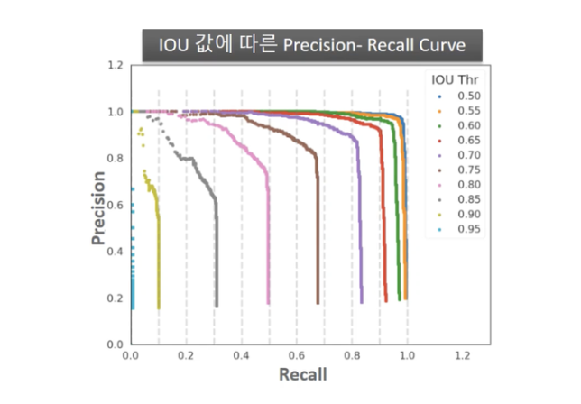
• 예측 성공을 위한 IOU를 0.5 이상으로 고정한 PASCAL VOC와 달리 COCO Challenge는 IOU 를 다양한 범위로 설정하여 예측 성공 기준을 정함.
• IOU 0.5부터 0.05씩 증가 시켜 0.95까지 해당하는 IOU별로 mAP를 계산
• 또한 크기의 유형(대/중/소)에 따른 mAP도 측정