기초

1. 정의: 여러개의 이미지로 분할하는 과정
2. 활용: object classification(물체 분류)
3. 입출력
   1. 입력: gray-sclae 이미지
   2. 출력: binary image(0과 255또는 0과 1 같이 2개의 값으로만 이루어진 값)

thresholding(임계처리)

1. 영상 분할 기법 중 하나

2. 가정
   1. 분할, 추출하고 싶은 물체와 배경의 밝기값 다름
   2. 배경영역과 물체 영역 내의 밝기값이 단조로움(차이가 별로 없음)
   

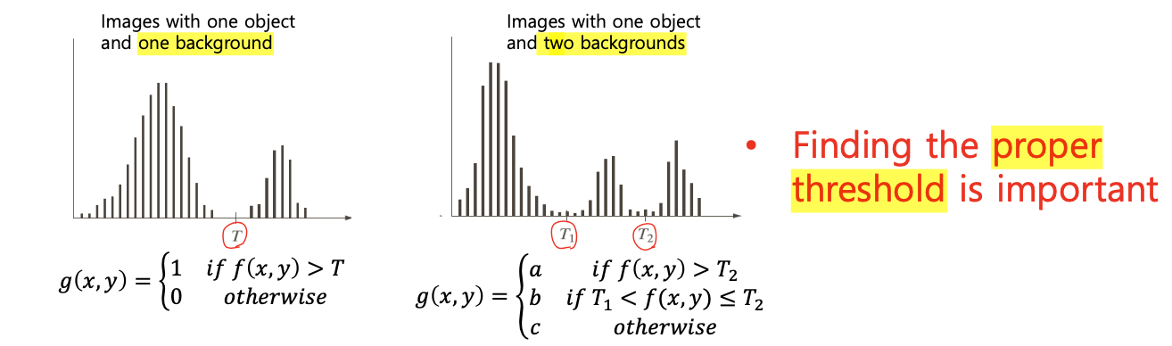
   적절한 threshold를 찾는 것이 중요

3. 유의점

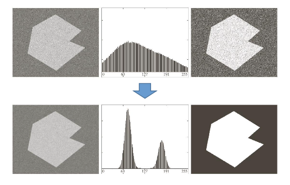
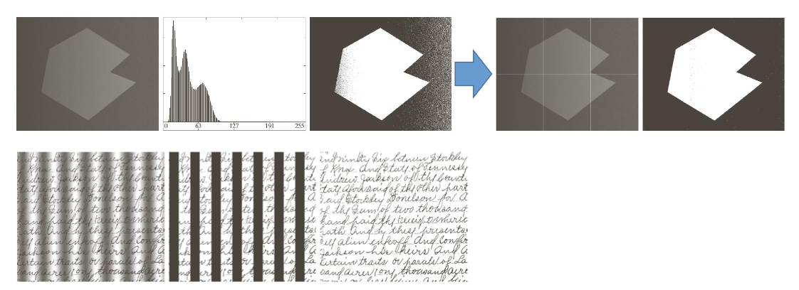
   1. noise(노이즈)
   2. illumination and reflectance(조명과 반사)
   3. 위와 같은 문제를 해결하기 위해 thresholding 이전에 smoothing을 적용
      

4. 종류

   1. global thresholding: 각 픽셀마다 같은 threshold 사용

      1. 기본 방식

         1. 초기 임의의 threshold T설정
         2. t로 segmentation 수행하여 2개의 그룹으로 나눔
         3. 각 그룹에 대해 픽셀들의 평균값 m1, m2 구함
         4. m1, m2로 새로운 threshold 구함 T = 0.5X(m1+m2) -> 어떤 의미인가?
         5. 이 2개의 t가 유사하다면 종료, 그렇지 않다면(차이가 크다면) 새로 구한 t를 가지고 2~4번 반복

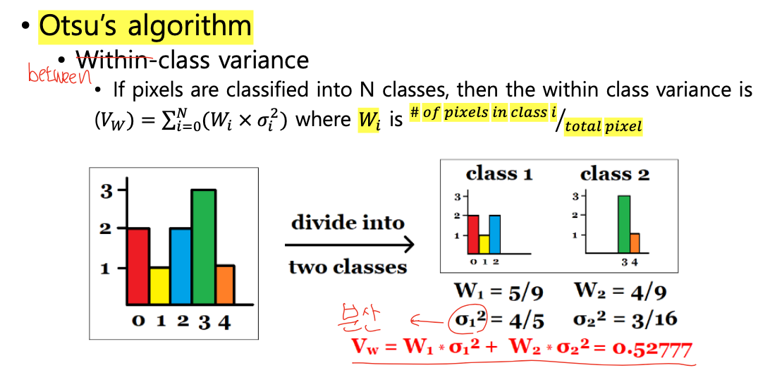
      2. othu's method

         1. 개념

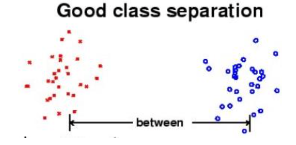
         2. 좋은 threshold를 가지고 하나의 영상을 두개의 그룹으로 분할 하였다면 --> 두 그룹의 밝기 차이는 큼, 하나의 그룹에 속한 픽셀들의 값은 유사

         3. 즉, 다양한 t를 적용해보았을 때 픽셀값의 차이가 크다면 이 t는 좋은 t임 --> T를 사용하겠다는 의미

         4. 이미지 히스토그램으로 판단
            

         5. 방식

            1. 영상에 대하여 nomalized histogram을 구함
            2. T의 후보인 k의 between class-variance(두 영역의 밝기 차이)를 계산
            3. 즉, k는 between class-variance가 max일 때로 선택

   2. local thresgholding: 각 픽셀마다 다른 threshold 사용

      1. 각각의 픽셀에 대한 t를 정할 때, 주변의 픽셀값들의 분포를 토대로 구함
         1. 종류
            1. ADAPTIVE_THRESH_MEAN_C : 𝑇 (𝑥, 𝑦) = 𝑚𝑒𝑎𝑛 𝑜𝑓 𝑡ℎ𝑒 𝑏𝑙𝑜𝑐𝑘𝑠𝑖𝑧𝑒 × 𝑏𝑙𝑜𝑐𝑘𝑠𝑖𝑧𝑒 𝑛𝑒𝑖𝑔ℎ𝑏𝑜𝑟ℎ𝑜𝑜𝑑 𝑜𝑓 (𝑥, 𝑦) − 𝐶 (주변 픽셀들의 평균- 상수C) --> 이 값이 threshold(문턱값이 됨), 해당 픽셀에 대해서 thresholding 수행
            2. ADAPTIVE_THRESH_GAUSSIAN_C : 𝑇 (𝑥, 𝑦) = 𝑎 𝑤𝑒𝑖𝑔ℎ𝑡𝑒𝑑 𝑠𝑢𝑚(𝑐𝑟𝑜𝑠𝑠 − 𝑐𝑜𝑟𝑟𝑒𝑙𝑎𝑡𝑖𝑜𝑛 𝑤𝑖𝑡ℎ 𝑎 𝐺𝑎𝑢𝑠𝑠𝑖𝑎𝑛 𝑤𝑖𝑛𝑑𝑜𝑛𝑤) 𝑜𝑓 𝑡ℎ𝑒 𝑏𝑙𝑜𝑐𝑘𝑠𝑖𝑧𝑒 × 𝑏𝑙𝑜𝑐𝑘𝑠𝑖𝑧𝑒 𝑛𝑒𝑖𝑔ℎ𝑏𝑜𝑟ℎ𝑜𝑜𝑑 𝑜𝑓 (𝑥, 𝑦) − 𝐶 (가우시안 함수를 활용해서 가중치 평균을 구한 후, 거기서 특정한 상수 C값을 뺌)
         2. image partitioning: 임의로 영상을 분할해서, 각 분할된 영역별로 thresholing 할 수 있음
            

5. 코드

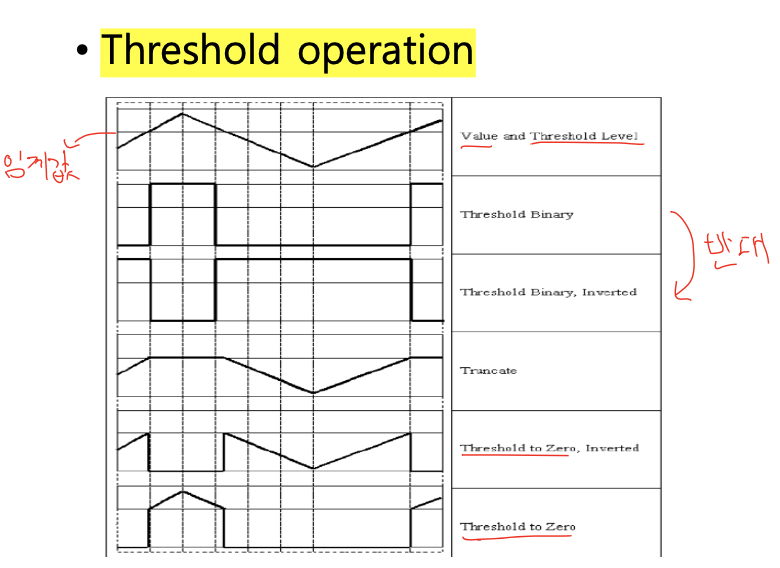
Threshold operation -->

double threshold (Mat src, Mat dst, double thresh, double maxval, int type)
• Apply fixed level thresh to each array element
• Typically used to get binary image from grayscale input image
• maxval : dst(I) = maxval if src(I) > thresh, 0 otherwise, when type is THRESH_BINARY
• Type : THRESH_BINARY, THRESH_BINARY_INV, THRESH_TRUNC, THRESH_TOZERO, THRESH_TOZERO_INV

int main() {

  Mat image = imread("lena.png");
  cvtColor(image, image, CV_BGR2GRAY);
  Mat dst;
  threshold(image, dst, 100, 255, THRESH_BINARY);
  
  imshow("dst", dst); 
  imshow("image", image); 
  waitKey(0);
  return 0;
}

void adaptiveThreshold(Mat src, Mat dst, double maxval, int adaptiveMethod, int thresholdType, int blockSize, double C)
• adaptiveMethod:ADAPTIVETHRESH_MEAN_C, ADAPTIVETHRESH_GAUSSIAN_C
• thresholdType:THRESH_BINARY,THRESH_BINARY_INV
• blockSIze : size of neighborhood used to calculate threshold (3,5,7)
• C : constant subtracted from mean or weighted mean
• dst(x, y) is computed as MEAN(blockSize x blockSize)-C or GAUSSIAN(blockSize x blockSize) –C around (x,y)

int main() {
  Mat image = imread("lena.png");
  cvtColor(image, image, CV_BGR2GRAY);
  Mat dst;
  
  adaptiveThreshold(image, dst, 255, ADAPTIVE_THRESH_MEAN_C, THRESH_BINARY, 7, 10); 
  imshow("dst", dst);
  imshow("image", image);
  
  waitKey(0);
  return 0;
}

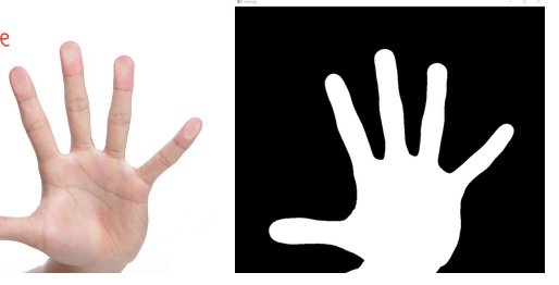
Void inRange(cv::InputArray src, cv::InputArray lowerb, cv::InputArray upperb, cv::OutputArray dst)
• src – first input array.
• lowerb – inclusive lower boundary array or a scalar
• upperb – inclusive upper boundary array or a scalar
• dst – output array of the same size as src and CV_8U type

int main() {

  Mat image = imread("hand.png");
  
  cvtColor(image, image, CV_BGR2YCrCb); 
  inRange(image, Scalar(0, 133, 77), Scalar(255, 173, 127), image);
  imshow("inRange", image); // 사이의 값들 --> white, 사이 값x --> black

  
  waitKey(0);
  return 0;
  
}

--> Global Thresholding

1. basic method

int main() {
  Mat image, thresh;
  int thresh_T, low_cnt, high_cnt, low_sum, high_sum, i, j, th;  
  
  thresh_T = 200;
  th = 10;
  low_cnt = high_cnt = low_sum = high_sum = 0;
  
  image = imread("lena.png", 0);
  cout << "threshold value:" << thresh_T << endl;
  
  while (1) {
  
    for (j = 0; j < image.rows; j++) {
      for (i = 0; i < image.cols; i++) {
        if (image.at<uchar>(j, i) < thresh_T) {
          low_sum += image.at<uchar>(j, i);
          low_cnt++; 
        }
        else {
          high_sum += image.at<uchar>(j, i);
          high_cnt++; 
        }
      }
    }  
    
    if (abs(thresh_T - (low_sum / low_cnt + high_sum / high_cnt) / 2.0f) < th) {
    	break; 
    }
    else {
      thresh_T = (low_sum / low_cnt + high_sum / high_cnt) / 2.0f; cout << "threshold value:" << thresh_T << endl;
      low_cnt = high_cnt = low_sum = high_sum = 0;
		} 
	}

  threshold(image, thresh, thresh_T, 255, THRESH_BINARY);
  
  imshow("Input image", image); 
  imshow("thresholding", thresh); 
  waitKey(0);
}
    

2. otsu's algorithm
   W:weigt(가중치-전체 중)와 M:mean(평균)은 다름

int main() {
  Mat image, result;
  
  image = imread("lena.png", 0);
  threshold(image, result, 0, 255, THRESH_BINARY | THRESH_OTSU);
  imshow("Input image", image);
  imshow("result", result);
  
  waitKey(0); 
 }

Local(Adaptive) Thresholding

int main() {

  Mat image, binary, adaptive_binary; 
  image = imread("opencv.jpg", 0);
  
  threshold(image, binary, 150, 255, THRESH_BINARY); // globla thresholding
  adaptiveThreshold(image, adaptive_binary, 255, ADAPTIVE_THRESH_MEAN_C, THRESH_BINARY, 85, 15); // local thresholding
  
  imshow("Input image", image); 
  imshow("binary", binary);
  imshow("adaptive binary", adaptive_binary); 
  waitKey(0);
  
}

grabcut

1. 개념
   1. 사용자와의 최소한의 상호작용으로 객체 추출을 실행
2. 절차
   1. 직사각형 입력 --> 직사각형 밖은 배경으로 인식, 안쪽은 미결정 상태
   2. 주어진 정보로 컴퓨터 초기 labelling 진행 --> foregfound와 background 픽셀 구별
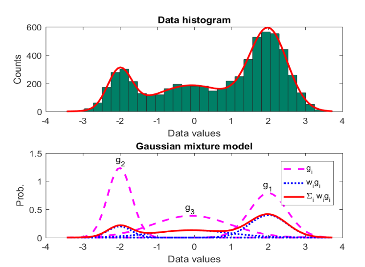
   3. GMM(Gaussian Mixture Model) 이용 --> foreground와 background model함
      1. Conditional probabilities
         1. 𝑝 (𝐴 ∩ 𝐵) = 𝑝 (𝐴|𝐵) 𝑝 (𝐵) = 𝑝(𝐵|𝐴)𝑝(𝐴)
      2. Bayes rule
         
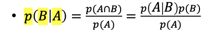
      3. Assume A is pixel value, and B is background
         
         
   4. GMM 이용하여 픽셀 분할 --> 미결정 픽셀 probalbe foreground와 pobable background로 label
   5. 이 픽셀 분포로부터 그래프 작성, 픽셀은 그래프 노드가 됨
   6. foreground pixel --> source node, background pixel --> sink node에 연결
      1. 픽셀이 foreground 또는 background일 확률에 의해 source node와 sink node와의 엣지 가중치 결정
      2. 엣지 가중치는 엣지 정보와 픽셀 유사도에 의해 결정 --> 픽셀 차이가 크면 낮은 엣지 가중치를 가짐
   7. mincut(minimum cost function) 알고리즘 통해 그래프 source node와 sink node로 자름
   8. cut 이후 source node는 물체, sink node는 배경이 됨
   9. 분류 완료할 때까지 프로세스 반복
3. 코드

   void grabCut(cv::InputArray img, cv::InputOutputArray mask, cv::Rect rect, cv::InputOutputArray bdgModel, cv::InputOutputArray fgdModel, int iterCount, int mode)
   • img - Input image
   • mask - mask image specifying background, foreground
   • rect - Coordinates of squares with foreground
   • bdgModel, fgdModel - Array used internally by algorithm
   • iterCount - Number of iterations the algorithm must run
   • mode - There are two types, GC_INIT_WITH_RECT and GC_INIT_WITH_MASK, each using a rectangle or mask to perform this algorithm

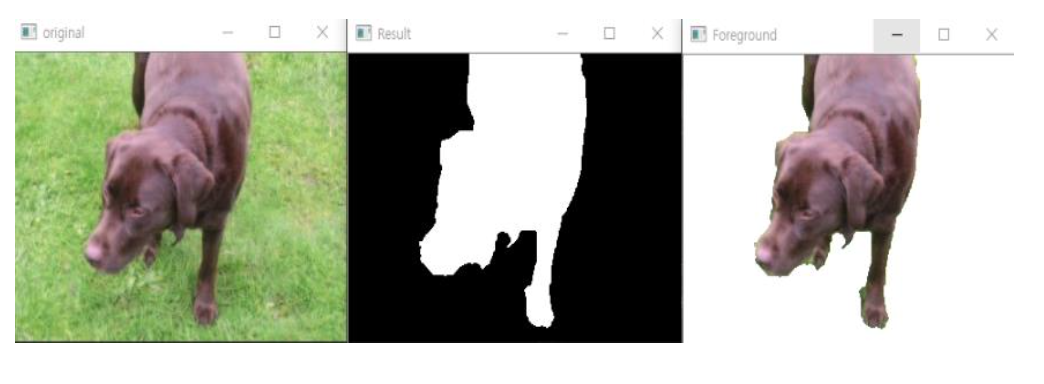
int main() {
  Mat result, bgdModel, fgdModel, image, foreground;
  image = imread("dog.png");
  //inner rectangle which includes foreground
  Rect rectangle(15, 0, 155, 240); // rectangle 크기
  
  grabCut(image, result, rectangle, bgdModel, fgdModel, 10, GC_INIT_WITH_RECT); compare(result, GC_PR_FGD, result, CMP_EQ);
  foreground = Mat(image.size(), CV_8UC3, Scalar(255, 255, 255)); image.copyTo(foreground, result);
  
  imshow("original", image);
  imshow("Result", result);
  imshow("Foreground", foreground);
  
  waitKey(0);
}