[ML] Perceptron (with Scikit-learn)

scikit-learn 으로 Perceptron training

의존성 설치

 pipenv install scikit-learn numpy
 pipenv install matplotlib

dataset training

• train_test_split : 데이터셋을 training/test 데이터셋으로 분리
  • test_size : 전체 데이터셋 중 test 데이터셋 비율
  • stratify : stratification (계층화) 수행
    • training 데이터셋과 test 데이터셋의 class label 비율을 input 데이터셋과 동일하게 함

• StandardScaler

  • fit : 입력된 데이터셋에 대해 feature dimension 마다 평균과 표준 편차 계산
    • ex) sc.fit(x_train)
  • transform : 입력된 데이터셋에 대해 평균과 표준 편차로 표준화하여 데이터셋 리턴
    x_train_std = sc.transform(x_train)
    x_test_std = sc.transform(x_test)

• Perceptron 클래스

  • max_iter : epoche (훈련 반복 횟수) 정의
  • fit: perceptron 모델 training
  • predict : class label 예측
  • score : 예측 + 스코어 계산을 시행하여 정확도 계산

• accuracy_score 메소드 : class label 예측 결과를 비교하여 정확도 계산

from sklearn import datasets
from sklearn.model_selection import train_test_split
from sklearn.preprocessing import StandardScaler
from sklearn.linear_model import Perceptron
from sklearn.metrics import accuracy_score
from matplotlib.colors import ListedColormap
import matplotlib.pyplot as plt
import numpy as np


def train_perceptron():
    """
    iris(붓꽃) 데이터셋으로 꽃받침 길이, 꽃잎 길이 2개 feature 로 분류하기
    :return:
    """
    iris_dataset = datasets.load_iris()
    x = iris_dataset.data[:, [2, 3]] # 꽃 데이터셋 중 일부 feature 만 추출 (꽃받침, 꽃길이)
    y = iris_dataset.target # 꽃 품종 label

    # test_size : test data와 training data 비율. 0.3이면 test 30%, training 70%
    # random_state: 데이터셋을 섞기 위해 사용되는 random seed. 고정일 경우 매번 동일하게 재현
    # stratify : stratification (계층화). training, test 데이터 셋의 label 비율을 input 데이터셋과 동일하게 함
    x_train, x_test, y_train, y_test = train_test_split(x, y, test_size=0.3, random_state=1, stratify=y)

    print(f'class label : {np.unique(y)}')

    # stratification 결과 체크
    print(f'y original data set label count : {np.bincount(y)}')
    print(f'y training data set label count : {np.bincount(y_train)}')
    print(f'y test data set label count : {np.bincount(y_test)}')

    # feature 표준화
    sc = StandardScaler()
    # traing data set 의 feature dimension 마다 평균과 표준 편차 계산
    sc.fit(x_train)

    # transform: 평균과 표준 편차로 data set 을 표준화
    x_train_std = sc.transform(x_train)
    x_test_std = sc.transform(x_test)

    # eta0 : learning rate
    # max_iter : epoch (traing 반복 최대 횟수) default 1000
    ppn = Perceptron(eta0=0.1, random_state=1, max_iter=1000)
    ppn.fit(x_train_std, y_train)

    # training 후 예측
    # y_test: true class label
    # y_predicted : predicted class label (예측한 label)
    y_predicted = ppn.predict(x_test_std)
    print(f'y_test      : {y_test}')
    print(f'y_predicted : {y_predicted}')
    print(y_test != y_predicted)
    print(f'분류 잘못된 샘플 수 {(y_test != y_predicted).sum()}')

    print(f'분류 오차 : {(y_test != y_predicted).sum() / len(y_test) * 100:.3f} %')
    print(f'정확도(accuracy) : {accuracy_score(y_test, y_predicted):.3f}')
    print(f'정확도(accuracy) : {ppn.score(x_test_std, y_test):.3f}')  # predict 와 accuracy_score 를 합쳐 정확도 계산

• 출력값

class label : [0 1 2]
y original data set label count : [50 50 50]
y training data set label count : [35 35 35]
y test data set label count : [15 15 15]
y_test      : [2 0 0 2 1 1 2 1 2 0 0 2 0 1 0 1 2 1 1 2 2 0 1 2 1 1 1 2 0 2 0 0 1 1 2 2 0
 0 0 1 2 2 1 0 0]
y_predicted : [2 0 0 2 1 1 2 1 2 0 0 2 0 1 0 1 2 1 1 2 2 0 1 2 1 1 0 2 0 2 0 0 1 1 2 2 0
 0 0 1 2 2 1 0 0]
[False False False False False False False False False False False False
 False False False False False False False False False False False False
 False False  True False False False False False False False False False
 False False False False False False False False False]
분류 잘못된 샘플 수 1
분류 오차 : 2.222 %
정확도(accuracy) : 0.978
정확도(accuracy) : 0.978

시각화 함수 정의

def plot_decision_regions(x, y, classifier, test_idx=None, resolution=0.02):
    """
    시각화
    :param x: 붓꽃 데이터셋 feature (0번 열 : 꽃받침 길이, 1번 열 : 꽃잎 길이)
    :param y: class label
    :param classifier: 분류기
    :param test_idx:
    :param resolution:
    :return:
    """
    # 마커, 컬러맵 설정
    markers = ('s', 'x', 'o', '^', 'v')
    colors = ('red', 'blue', 'lightgreen', 'gray', 'cyan')
    cmap = ListedColormap(colors[:len(np.unique(y))])

    # decision boundary (결정 경계) 그리기
    # feature
    x1_min, x1_max = x[:, 0].min() - 1, x[:, 0].max() + 1 # feature column 0 -> 꽃받침 길이
    x2_min, x2_max = x[:, 1].min() - 1, x[:, 1].max() + 1 # feature column 1 ->  꽃잎 길이

    # meshgrid : 축에 해당하는 1차원 배열을 받아 벡터 공간의 모든 좌표를 담은 행렬을 반환
    xx1, xx2 = np.meshgrid(np.arange(x1_min, x1_max, resolution), 
                           np.arange(x2_min, x2_max, resolution))
    # ravel : 배열을 1차원 배열로 펼치기
    # T : transpose
    # 2개 배열을 펼치고 각 행으로 붙이고 transpose 하여 2개의 열로 변환, 이후 class label 예측
    z = classifier.predict(np.array([xx1.ravel(), xx2.ravel()]).T)
    # xx1, xx2 와 같은 차원의 그리드로 크기 변경
    z = z.reshape(xx1.shape)
    # contourf : 등고선 그래프 그리기
    plt.contourf(xx1, xx2, z, alpha=0.3, cmap=cmap)
    # x, y축 limit 설정
    plt.xlim(xx1.min(), xx1.max())
    plt.ylim(xx2.min(), xx2.max())

    for idx, cl in enumerate(np.unique(y)):
        plt.scatter(x=x[y == cl, 0], y=x[y == cl, 1],
                    alpha=0.8, c=colors[idx],
                    marker=markers[idx], label=cl,
                    edgecolor='black')

    if test_idx:
        x_test, y_test = x[test_idx, :], y[test_idx]

    plt.scatter(x_test[:, 0], x_test[:, 1],
                facecolors='none', edgecolor='black', alpha=1.0,
                linewidth=1, marker='o',
                s=100, label='test_set')

• training 후 시각화
  • 위 training 코드와 이어짐

    # 시각화를 위해 training, test data set 결합
    x_combined_std = np.vstack((x_train_std, x_test_std))
    y_combined = np.hstack((y_train, y_test))

    # 시각화
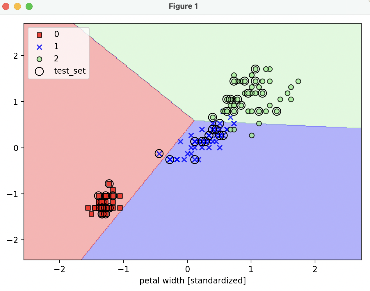
    plot_decision_regions(x=x_combined_std, y=y_combined, classifier=ppn, test_idx=range(105,150))
    plt.xlabel('petal length [standardized]')
    plt.xlabel('petal width [standardized]')
    plt.legend(loc='upper left')
    plt.tight_layout()
    plt.show()

• 그러나, perceptron 으로는 decision boundary 로 명확하게 분류되지 않는다.
  • perceptron 은 선형 분류기이기 때문에, 비선형 문제에 대해선 한계가 있어 잘 사용되지 않는다.

reference

• 서적 '머신러닝 교과서 with 파이썬, 사이킷런, 텐서플로 개정 3판'