[Pytorch] Object Detection Model 구현하기

Object Detection Model 구현

Pytorch를 이용하여 Object Detection Model을 구현해볼 것이다. YOLOv1 Network를 직접 구축할 것이며, 데이터셋은 VOC 2007과 VOC 2012를 더한 형태의 데이터셋을 사용할 것이다. 이때 빠른 학습을 위해 이미지의 수를 줄이고, 클래스 또한 6개로 축소할 것이다.
다른 알고리즘들은 Bounding Box를 찾고 Class를 분류하고 Confidence Score를 찾는 과정을 따로 진행했다면, YOLO는 단 한번의 Regression으로 이 모든 output을 찾게된다. 따라서 YOLO를 사용하면 어떤 물체가 있고 어디에 있는지 예측하기 위해 이미지를 한 번만 보게 된다.

YOLO는 Input Image를 S X S grid로 나누고 각각의 grid 셀마다 B개의 Bounding Box를 예측한다.(각 Bounding Box는 x, y, w, h, Confidence 총 5가지의 숫자로 구성된다.)
이렇게 되면 Bounding Box는 총 SXSXB개가 생성된다. 이후 NMS 기법을 통해 가장 높은 신뢰도를 지니는 Box만 남긴다. 그리고 Class들에 대한 점수를 통해 가장 높은 점수를 가진 Class를 Box의 Class로 결정한다.
이때, 모든 점수가 0에 가까우면 해당 Box에는 객체가 존재하지 않거나 판별할 수 없는 경우이므로 Box를 삭제한다.

이 과정들을 거치면 위 이미지의 Final detections 처럼 객체를 판별하는 Box만 남게 된다.

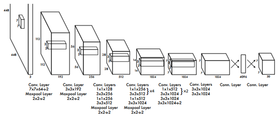위 이미지는 YOLOv1 Network의 Architecture이다. 24개의 Convolutional Layer와 2개의 Fully Connected Layer로 이루어져 있다.

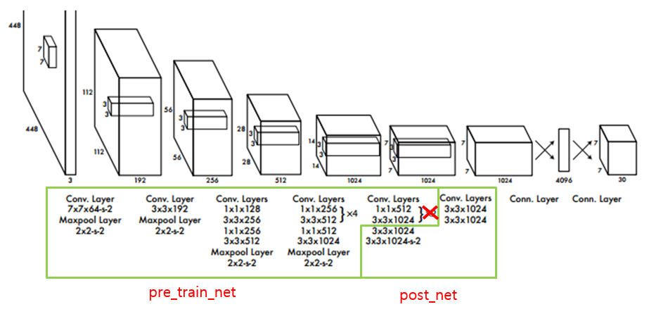여기서 이 Architecture를 pre_train_net, post_net으로 나눠줄 것이다. 그리고 2개의 Convolutional Layer를 삭제하여 22개의 Convolutional Layer로 축소해준다. 이는 ImageNet dataset으로 Pre-trained된 network와 구조를 맞춰주기 위한 것이다.

활성화 함수는 LeakyReLU(Leaky Rectified Linear Unit)를 사용할 것이다. LeakyReLU는 기본 ReLU 함수의 변형된 형태로, 수학적 표현은 아래와 같다.
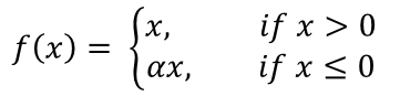$x$ 는 입력 값이고, $α$는 아주 작은 상수이다. 이 상수 값은 음수 입력에 대한 출력의 기울기를 결정한다. 음수 입력에 대해 작은 기울기를 허용함으로써 학습 도중 가중치 업데이트가 중단되는 경우를 방지할 수 있다.

YOLOv1에서 사용된 Loss function은 아래와 같다.

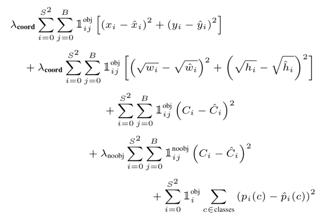여기서 $1_{obj}$은 ground truth box의 중심이 Grid cell $i$에 있는지를 보여주는 indicator function이다. Object가 Grid cell $i$와 $j$번째 Bounding Box Predictor에 존재할 경우 값이 1이고, 이 외에는 0의 값이다.
이 Loss function은 하나의 predictor가 ground truth에 대해 가장 높은 IoU를 갖는 object를 예측할 수 있도록 해준다.
$λ_{coord}$와 $λ_{noobj}$는 논문과 동일하게 각각 5와 0.5로 설정할 것이다.
Loss function은 크게 3개의 파트로 나눌 수 있다.

1.
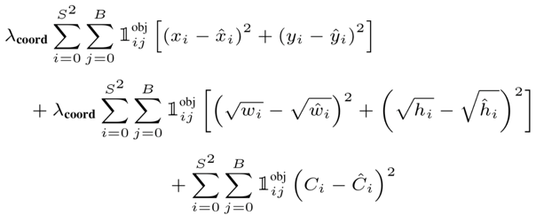Bounding Box 좌표 $(x, y, w, h)$를 Regression하고, Object Confidence에 대한 loss를 부과하는 파트이다. 예측된 Bounding Box 좌표 $(x, y)$와 width/height $(w, h)$에 대한 loss를 계산한다.
이때 width와 height는 제곱근을 통해 조정되게 된다. 이는 큰 상자에서의 Bounding Box 오차에 더 큰 loss를 부여하기 위해서이다. 그리고 Cell 내의 Object에 대한 Confidence Score의 loss를 계산한다.

2.
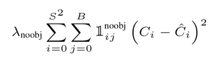Bounding Box Predictor와 관련된 Confidence Score와 관련된 loss를 계산하는 파트이다. $λ_{noobj}$ cell에 Object가 없다면 1이고, 그렇지 않으면 0이다.

3.
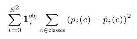Classification과 관련된 파트이다. cell 안에 Object가 없으면 Classifiction error에 페널티를 주지 않는다.

이제 본격적으로 코드를 통해 Object Detection Model(YOLOv1)을 구현해볼 것이다.

---

Import

우선 필요한 것들을 import 해준다.

import torch
import torch.nn as nn
import torch.nn.functional as F
import torch.optim as optim
from torch.utils.data import DataLoader

import function

import math

from util import *

---

Model

모델을 구현해준다. 이전에 수정했던것 처럼 22개의 Convolutional Layer를 pre_train_net과 post_net으로 나눠서 구성해준다. 그리고 2개의 Fully Connected Layer를 추가해준다.

class YOLOv1(nn.Module):
    def __init__(self):
        super(YOLOv1, self).__init__()

        self.pre_train_net = nn.Sequential(
            nn.Conv2d(in_channels=3, out_channels=64, kernel_size=7, stride=2, padding=3),
            nn.LeakyReLU(negative_slope=0.01),
            nn.MaxPool2d(kernel_size=2, stride=2),

            nn.Conv2d(in_channels=64, out_channels=192, kernel_size=3, stride=1, padding=1),
            nn.LeakyReLU(negative_slope=0.01),
            nn.MaxPool2d(kernel_size=2, stride=2),

            nn.Conv2d(in_channels=192, out_channels=128, kernel_size=1, stride=1, padding=0),
            nn.LeakyReLU(negative_slope=0.01),

            nn.Conv2d(in_channels=128, out_channels=256, kernel_size=3, stride=1, padding=1),
            nn.LeakyReLU(negative_slope=0.01),

            nn.Conv2d(in_channels=256, out_channels=256, kernel_size=1, stride=1, padding=0),
            nn.LeakyReLU(negative_slope=0.01),

            nn.Conv2d(in_channels=256, out_channels=512, kernel_size=3, stride=1, padding=1),
            nn.LeakyReLU(negative_slope=0.01),
            nn.MaxPool2d(kernel_size=2, stride=2),

            nn.Conv2d(in_channels=512, out_channels=256, kernel_size=1, stride=1, padding=0),
            nn.LeakyReLU(negative_slope=0.01),

            nn.Conv2d(in_channels=256, out_channels=512, kernel_size=3, stride=1, padding=1),
            nn.LeakyReLU(negative_slope=0.01),

            nn.Conv2d(in_channels=512, out_channels=256, kernel_size=1, stride=1, padding=0),
            nn.LeakyReLU(negative_slope=0.01),

            nn.Conv2d(in_channels=256, out_channels=512, kernel_size=3, stride=1, padding=1),
            nn.LeakyReLU(negative_slope=0.01),

            nn.Conv2d(in_channels=512, out_channels=256, kernel_size=1, stride=1, padding=0),
            nn.LeakyReLU(negative_slope=0.01),

            nn.Conv2d(in_channels=256, out_channels=512, kernel_size=3, stride=1, padding=1),
            nn.LeakyReLU(negative_slope=0.01),

            nn.Conv2d(in_channels=512, out_channels=256, kernel_size=1, stride=1, padding=0),
            nn.LeakyReLU(negative_slope=0.01),

            nn.Conv2d(in_channels=256, out_channels=512, kernel_size=3, stride=1, padding=1),
            nn.LeakyReLU(negative_slope=0.01),

            nn.Conv2d(in_channels=512, out_channels=512, kernel_size=1, stride=1, padding=0),
            nn.LeakyReLU(negative_slope=0.01),

            nn.Conv2d(in_channels=512, out_channels=1024, kernel_size=3, stride=1, padding=1),
            nn.LeakyReLU(negative_slope=0.01),
            nn.MaxPool2d(kernel_size=2, stride=2),

            nn.Conv2d(in_channels=1024, out_channels=512, kernel_size=1, stride=1, padding=0),
            nn.LeakyReLU(negative_slope=0.01),

            nn.Conv2d(in_channels=512, out_channels=1024, kernel_size=3, stride=1, padding=1),
            nn.LeakyReLU(negative_slope=0.01)


        )

        self.post_net = nn.Sequential(
            nn.Conv2d(in_channels=1024, out_channels=1024, kernel_size=3, stride=1, padding=1),
            nn.LeakyReLU(negative_slope=0.01),

            nn.Conv2d(in_channels=1024, out_channels=1024, kernel_size=3, stride=2, padding=1),
            nn.LeakyReLU(negative_slope=0.01),

            nn.Conv2d(in_channels=1024, out_channels=1024, kernel_size=3, stride=1, padding=1),
            nn.LeakyReLU(negative_slope=0.01),

            nn.Conv2d(in_channels=1024, out_channels=1024, kernel_size=3, stride=1, padding=1),
            nn.LeakyReLU(negative_slope=0.01),
        )

        self.FC1 = nn.Sequential(
            nn.Linear(50176, 4096),
            nn.LeakyReLU(),
            nn.Dropout()
        )

        self.FC2 = nn.Sequential(
            nn.Linear(4096, 1470)
        )

        self.pre_train_net.cuda()
        self.post_net.cuda()
        self.FC1.cuda()
        self.FC2.cuda()

        self._initialize_weights()

    def forward(self, x):
        output = self.pre_train_net(x)
        output = self.post_net(output)

        # Fully Connected Layer에 통과시키기 위해 1차원 형태로 변환
        output = output.view(output.size(0), -1)

        output = self.FC1(output)
        output = self.FC2(output)
        
        # Shape: (batch_size, 7, 7, 30)
        output = output.view(output.size(0), 7, 7, 30)

        output = F.relu(output)

        return output

    # 가중치 초기화
    def _initialize_weights(self):
        for m in self.modules():
            if isinstance(m, nn.Conv2d):
                n = m.kernel_size[0] * m.kernel_size[1] * m.out_channels
                m.weight.data.normal_(0, math.sqrt(2. / n))
                if m.bias is not None:
                    m.bias.data.zero_()
            elif isinstance(m, nn.BatchNorm2d):
                m.weight.data.fill_(1)
                m.bias.data.zero_()
            elif isinstance(m, nn.Linear):
                m.weight.data.normal_(0, 0.01)
                m.bias.data.zero_()

---

Train

구현한 Model을 토대로 간단하게 학습을 진행해볼 것이다.
Loss function은 이전에 언급한 YOLO Loss function을 사용하고, Optimizer는 SGD(Stochastic Gradient Descent), Batch size와 Epoch는 10으로 설정한다.
ImageNet dataset으로 Pre-trained된 동일한 구조의 모델을 불러올 것이다.

train_dataset = function.YoloDataset(root='./all_img/', list_file='./Generate_dataset/voc2007+2012.txt', train=True)
train_loader = DataLoader(train_dataset, batch_size=10, shuffle=True, num_workers=4)

model = YOLOv1()
state_dict = torch.load('./pre_train.pt')
model.load_state_dict(state_dict['state_dict'])
print('pre_train_complete')

device = torch.device("cuda" if torch.cuda.is_available() else "cpu")
model.to(device)

optimizer = torch.optim.SGD(model.parameters(), lr=1e-3, momentum=0.9, weight_decay=5e-4)
optimizer.load_state_dict(state_dict['optimizer'])

criterion = function.yoloLoss(l_coord=5,l_noobj=0.5)

num_epochs = 10
print("training start")

for epoch in range(num_epochs):
    model.train()
    total_loss = 0

    for i, (images, target) in enumerate(train_loader):
        images = images.to(device)
        target = target.to(device)

        pred = model(images)
        loss = criterion(pred, target)

        total_loss += loss.item()

        optimizer.zero_grad()
        loss.backward()
        optimizer.step()

        if (i+1) % 10 == 0:
            print('Epoch [%d/%d], Iter [%d,%d] Loss:%.4f, average_loss: %.4f' % (epoch+1, num_epochs, i+1, len(train_loader), loss.item(), total_loss / (i+1)))

pre_train_complete
training start
Epoch [1/10], Iter [10,430] Loss:0.6008, average_loss: 0.6665
Epoch [1/10], Iter [20,430] Loss:0.5276, average_loss: 0.6811
Epoch [1/10], Iter [30,430] Loss:0.7125, average_loss: 0.6977
Epoch [1/10], Iter [40,430] Loss:0.4431, average_loss: 0.7223
Epoch [1/10], Iter [50,430] Loss:0.6330, average_loss: 0.7154
Epoch [1/10], Iter [60,430] Loss:0.8091, average_loss: 0.7129
Epoch [1/10], Iter [70,430] Loss:0.4213, average_loss: 0.6990
Epoch [1/10], Iter [80,430] Loss:0.7378, average_loss: 0.7054
Epoch [1/10], Iter [90,430] Loss:0.3034, average_loss: 0.6943
Epoch [1/10], Iter [100,430] Loss:0.3722, average_loss: 0.6779
Epoch [1/10], Iter [110,430] Loss:1.1623, average_loss: 0.6752
Epoch [1/10], Iter [120,430] Loss:0.9179, average_loss: 0.6779
Epoch [1/10], Iter [130,430] Loss:0.3683, average_loss: 0.6708
Epoch [1/10], Iter [140,430] Loss:0.3802, average_loss: 0.6647
Epoch [1/10], Iter [150,430] Loss:0.4768, average_loss: 0.6653
Epoch [1/10], Iter [160,430] Loss:0.7332, average_loss: 0.6650
Epoch [1/10], Iter [170,430] Loss:0.5728, average_loss: 0.6702
Epoch [1/10], Iter [180,430] Loss:1.0470, average_loss: 0.6693
Epoch [1/10], Iter [190,430] Loss:0.6120, average_loss: 0.6678
Epoch [1/10], Iter [200,430] Loss:0.7135, average_loss: 0.6764
Epoch [1/10], Iter [210,430] Loss:0.8442, average_loss: 0.6854
Epoch [1/10], Iter [220,430] Loss:0.7051, average_loss: 0.6854
Epoch [1/10], Iter [230,430] Loss:0.9952, average_loss: 0.6874
Epoch [1/10], Iter [240,430] Loss:0.3745, average_loss: 0.6813
Epoch [1/10], Iter [250,430] Loss:0.7021, average_loss: 0.6774
...
Epoch [10/10], Iter [400,430] Loss:0.5801, average_loss: 0.6179
Epoch [10/10], Iter [410,430] Loss:0.9818, average_loss: 0.6198
Epoch [10/10], Iter [420,430] Loss:0.6173, average_loss: 0.6201
Epoch [10/10], Iter [430,430] Loss:0.5707, average_loss: 0.6199

---

Predict

학습을 마친 Model을 통해 6개의 Class에 대해 Predict를 진행할 것이다.

function.visualize(model, './Generate_dataset/images/006412.jpg')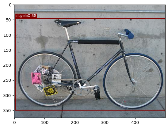

function.visualize(model, './Generate_dataset/images/000037.jpg')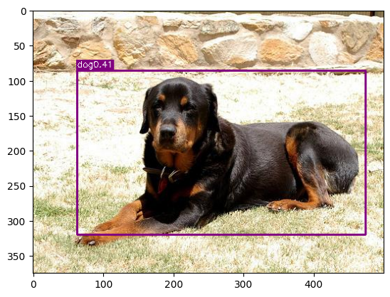

function.visualize(model, './Generate_dataset/images/000103.jpg')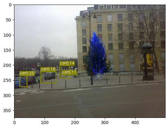

function.visualize(model, './Generate_dataset/images/000053.jpg')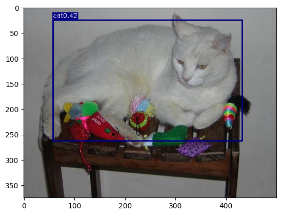

function.visualize(model, './Generate_dataset/images/006533.jpg')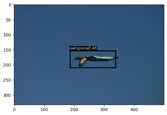

function.visualize(model, './Generate_dataset/images/006601.jpg')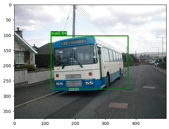

가장 최근의 YOLOv9 및 YOLOv10 모델 보다는 당연하게도 확실히 성능이 떨어지지만, Object의 Class와 위치를 어느정도 Detection 할 수 있는 것을 확인할 수 있다.