Seq2Seq with Attention
기존에 구현했던 Seq2Seq 모델에 Attention 메커니즘을 추가해볼 것이다. 이전 Seq2Seq 모델에 사용했던 것과 동일한 데이터셋을 사용할 것이다. 데이터셋에 대한 자세한 설명은 Seq2Seq 모델 구현 포스팅에 자세히 나와있다.
https://velog.io/@aurorab86/Pytorch-Seq2Seq-%EB%AA%A8%EB%8D%B8-%EA%B5%AC%ED%98%84#dataset
Import
필요한 것들을 import 한다.
import torch
import torch.nn as nn
import torch.optim as optim
import torch.nn.functional as F

import numpy as np

from collections import defaultdict

import matplotlib.pyplot as plt

from tqdm.auto import tqdm
Dataset
데이터셋 생성 함수를 구현한다.
def generate_data(seq_length_min=1, seq_length_max=20, batch_size=10):
    T = np.random.randint(seq_length_min, seq_length_max + 1)
    x = np.random.randint(0, 10, (T, batch_size))
    one_hot_x = np.zeros((T + 1, batch_size, 12), dtype=np.float32)
    one_hot_x[np.arange(T).reshape(-1, 1), np.arange(batch_size), x] = 1
    one_hot_x[-1, :, -1] = 1
    ends = np.full(batch_size, 11).reshape(1, -1)
    y = np.concatenate([x[::-1], ends], axis=0)
    return x, one_hot_x, y
그리고 추가적으로 가장 높은 점수를 가진 클래스에 해당하는 One-hot Encoding을 반환하는 함수를 미리 구현해준다.
def one_hot_encoding_prediction(y_t):
    """
    N : batch size
    K : 클래스 개수 (i.e. vocabulary의 크기)

    y_t: shape=(1, N, K)
        seq2seq 디코딩의 한 step으로부터 예측된 분류 점수

    one_hot_encoding: shape=(1, N, K)
        y_t에서의 가장 높은 점수에 해당하는 레이블에 1이 할당된 형태
    """
    y_t = y_t.detach().cpu().numpy()
    max_values_mask = (y_t == y_t.max(axis=-1, keepdims=True))
    one_hot_encoding = torch.tensor(max_values_mask.astype(np.float32), dtype=torch.float32)
    return one_hot_encoding
위 one_hot_encoding_prediction 함수의 동작 예시는 아래와 같다.
y_t = [[[0.1, 0.5, 0.3, 0.1],
        [0.2, 0.6, 0.1, 0.1],
        [0.0, 0.4, 0.1, 0.5]]]

max_values_mask = [[[False, True, False, False],
                    [False, True, False, False],
                    [False, False, False, True]]]

one_hot_encoding = torch.tensor([[[0.0, 1.0, 0.0, 0.0],
                                 [0.0, 1.0, 0.0, 0.0],
                                 [0.0, 0.0, 0.0, 1.0]]])
Model 구현 & 정의
Seq2Seq with Attention 모델과, 이에 필요한 RNN 모델을 구현한다. 설명은 주석을 활용하겠다.
class RNN(nn.Module):
    def __init__(self, dim_input, dim_recurrent, dim_output):
        super(RNN, self).__init__()

        """
        dim_input: C
        dim_recurrent: D
        dim_output: K
        """

        self.x2h = nn.Linear(dim_input, dim_recurrent)
        self.h2h = nn.Linear(dim_recurrent, dim_recurrent, bias=True)
        self.h2y = nn.Linear(dim_recurrent, dim_output)
        self.relu = nn.ReLU()

        nn.init.xavier_normal_(self.x2h.weight)
        nn.init.xavier_normal_(self.h2h.weight)
        nn.init.xavier_normal_(self.h2y.weight)

    def forward(self, x, h_t=None):

        """
        x: shape = (T, N, C)
        W_x: shape = (C, D)
        초기 h: shape = (1, N, D)
        W_h: shape = (D, D)

        => x X W_x: (T, N, C) X (C, D) = (T, N, D)
           (초기 h) X W_h: (1, N, D) X (D, D) = (1, N, D)

           h: (T, N, D) + (1, N, D) = (T, N, D) broadcasting

        w_y: shape = (D, K)

        y: h X w_y
         = (T, N, D) X (D, K) = (T, N, K)

        y: shape = (T, N, K)
        h: shape = (T, N, D)
        """

        N = x.shape[1]
        D = self.h2h.weight.shape[0]

        # 초기 hidden state를 (1, N, D) shape의 0텐서로 설정
        if h_t is None:
            h_t = torch.zeros(1, N, D, dtype=torch.float32)

        h = []

        for x_t in x:
            h_t = self.x2h(x_t.unsqueeze(0)) + self.h2h(h_t)
            h_t = self.relu(h_t)
            h.append(h_t)

        # 배열 h에 저장된 모든 hidden state들을 dim=0 방향으로 합치기
        all_h = torch.cat(h, dim=0)

        all_y = self.h2y(all_h)

        return all_y, all_h
class AttentionSeq2Seq(nn.Module):
def __init__(self, dim_input, dim_recurrent, dim_output):
super(AttentionSeq2Seq, self).__init__()
"""
dim_input: 입력 데이터 차원(C)
dim_recurrent: hidden state 차원(D)
dim_output: 디코더 출력 차원(K)
"""
self.encoder = RNN(dim_input, dim_recurrent, dim_output)
self.decoder = RNN(dim_input, dim_recurrent, dim_output)
"""
Attention 메커니즘을 적용하기 위해 dense layer를 추가로 생성
W_alpha: 인코더의 hidden state들에 가중치를 부여해주기 위해 생성
concat_dense: 이후에 디코더의 y_t와 Context vector c_t를 concatenate 해주기 위해 생성
"""
self.W_alpha = nn.Linear(dim_recurrent, dim_recurrent, bias=False)
self.concat_dense = nn.Linear(dim_recurrent + dim_output, dim_output)
nn.init.xavier_normal_(self.W_alpha.weight)
nn.init.xavier_normal_(self.concat_dense.weight)
def forward(self, x):
T, N, C = x.shape
y = []
# 인코더를 통해 hidden state를 받음, 인코더의 출력은 취급하지 않음
_, enc_h = self.encoder(x)
# 마지막 step에서의 hidden state를 지정
h_t = enc_h[-1:]
# <sos> 토큰 즉, 디코더 첫 step의 입력을 나타내는 start 토큰 설정
s_t = torch.zeros(1, N, C)
s_t[:, :, -2] = 1
# 인코더의 hidden state들을 W_alpha layer에 통과시켜 Attention Score의 일부를 미리 계산
precomputed_encoder_score_vectors = self.W_alpha(enc_h)
# 각 디코더 step에서의 Attention Weight를 저장하기 위해 생성
a_ij = []
# 타임스텝 T 동안 디코더 반복 실행
for _ in range(T):
# 우선 step을 진행하기 전에 현재 hidden state에 대한 Attention Score 계산
e_t = (precomputed_encoder_score_vectors*h_t).sum(dim=-1)
# 위에서 구한 Attention Score를 softmax 함수에 통과시켜 Attention Weight 도출
a_t = F.softmax(e_t, dim=0)
# Attention Weight를 리스트 a_ij에 저장
a_ij.append(a_t.unsqueeze(0))
# 인코더의 hidden state들과 Attention Weight를 통해 Context Vector 도출
c_t = (a_t[..., None]*enc_h).sum(dim=0, keepdims=True)
# 하나의 디코더 step을 진행(s_t, h_t 입력)하여 y_t와 h_t를 받음
y_t, h_t = self.decoder(s_t, h_t)
# 도출된 y_t와 이전에 구한 Context Vector를 dim=-1 방향으로 concatenate
y_and_c = torch.cat([y_t, c_t], dim=-1)
# concatenate된 벡터를 concat_dense layer에 통과시켜 새로운 y_t를 도출한 후 y에 저장
y_t = self.concat_dense(y_and_c)
y.append(y_t)
# 디코더의 다음 step의 입력값을 새로 할당
s_t = one_hot_encoding_prediction(y_t)
# 리스트 y에 저장된 모든 y들을 dim=0 방향으로 합치기
y = torch.cat(y, dim=0)
# 리스트 a_ij에 저장된 모든 Attention Weight들을 dim=0 방향으로 합치기
a_ij = torch.cat(a_ij, dim=0)
return y, a_ij model = AttentionSeq2Seq(dim_input=12, dim_recurrent=25, dim_output=12)
optimizer = optim.Adam(model.parameters())
modelAttentionSeq2Seq(
(encoder): RNN(
(x2h): Linear(in_features=12, out_features=25, bias=True)
(h2h): Linear(in_features=25, out_features=25, bias=True)
(h2y): Linear(in_features=25, out_features=12, bias=True)
(relu): ReLU()
)
(decoder): RNN(
(x2h): Linear(in_features=12, out_features=25, bias=True)
(h2h): Linear(in_features=25, out_features=25, bias=True)
(h2y): Linear(in_features=25, out_features=12, bias=True)
(relu): ReLU()
)
(W_alpha): Linear(in_features=25, out_features=25, bias=False)
(post_concat_dense): Linear(in_features=37, out_features=12, bias=True)
)모델을 AttentionSeq2Seq로 정의해준다. input과 output의 차원은 동일하게 12로 설정해주고, hidden state의 차원은 25로 설정해준다. 옵티마이저는 Adam을 사용한다.
Train
우선 Train 과정과 결과를 시각화하기 위한 함수를 구현해준다.
from IPython.display import clear_output
def plot_all(losses, acces):
    clear_output(wait=True)
    plt.figure(figsize=(10, 5))
    plt.plot(losses, label='Loss')
    plt.plot(acces, label='acc')
    plt.xlabel('Batches (It must multiple x 1000)')
    plt.ylabel('Loss and Acc')
    plt.title('Loss and Acc Averages over Epochs')
    plt.legend()
    plt.grid()
    plt.show()
이제 Train을 위한 loop를 구현해준다.
batch_size = 100
num_batches = 30000

losses = []
accs = []
lossesaverage_list = []
accslist_average = []
for k in range(num_batches):
    sequence, x, target  = generate_data(batch_size=batch_size)

    x_tensor = torch.tensor(x, dtype=torch.float32)
    target_tensor = torch.tensor(target, dtype=torch.long)

    optimizer.zero_grad()
    output, _ = model(x_tensor)

    lossesfn = nn.CrossEntropyLoss()
    loss = lossesfn(output.reshape(-1, 12), target_tensor.reshape(-1))
    loss.backward()
    optimizer.step()

    acc = (output.argmax(dim=-1) == target_tensor).float().mean().item()

    losses.append(loss.item())
    accs.append(acc)
    if k % 1000 == 0:
        accsaverage = np.mean(accs)
        lossesaverage = np.mean(losses)
        lossesaverage_list.append(lossesaverage)
        accslist_average.append(accsaverage)
        plot_all(lossesaverage_list, accslist_average)
        print(f"loss: {lossesaverage}, accuracy: {accsaverage}")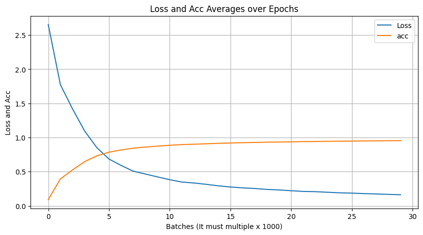
loss: 0.16111198735101503, accuracy: 0.9542968195647362Test
Train을 마친 Model을 통해 Test를 진행한다.
length_total = defaultdict(int)
length_correct = defaultdict(int)

with torch.no_grad():
    for i in tqdm(range(50000)):
        if i % 5000 == 0:
            print(f"{i}번 Test")
        if i == 50000:
            print(f"{i}번 Test")
        # Test를 위한 데이터셋을 따로 생성(batch_size는 1로 지정)
        sequence, x, target  = generate_data(1, 20, 1)

        x_tensor = torch.tensor(x, dtype=torch.float32)
        target_tensor = torch.tensor(target, dtype=torch.long)

        output, _ = model(x_tensor)

        length_total[sequence.size] += 1
        if (output.argmax(dim=-1) == target_tensor).all():
            length_correct[sequence.size] += 1

fig, ax = plt.subplots()
x, y = [], []
for i in range(1, 20):
    x.append(i)
    y.append(length_correct[i] / length_total[i])
ax.plot(x, y)0번 Test
5000번 Test
10000번 Test
15000번 Test
20000번 Test
25000번 Test
30000번 Test
35000번 Test
40000번 Test
45000번 Test
49999번 Test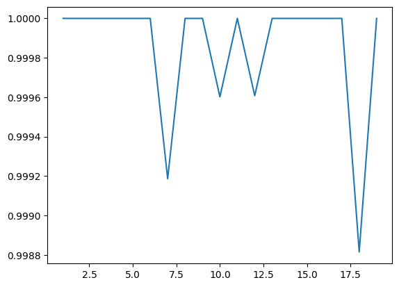 x축은 Sequence의 길이이고, y축은 Sequence 길이에 따른 Accuracy 값이다. 이 결과를 Attention 메커니즘을 적용하지 않은 Seq2Seq 모델의 결과와 비교하면 어떨까?
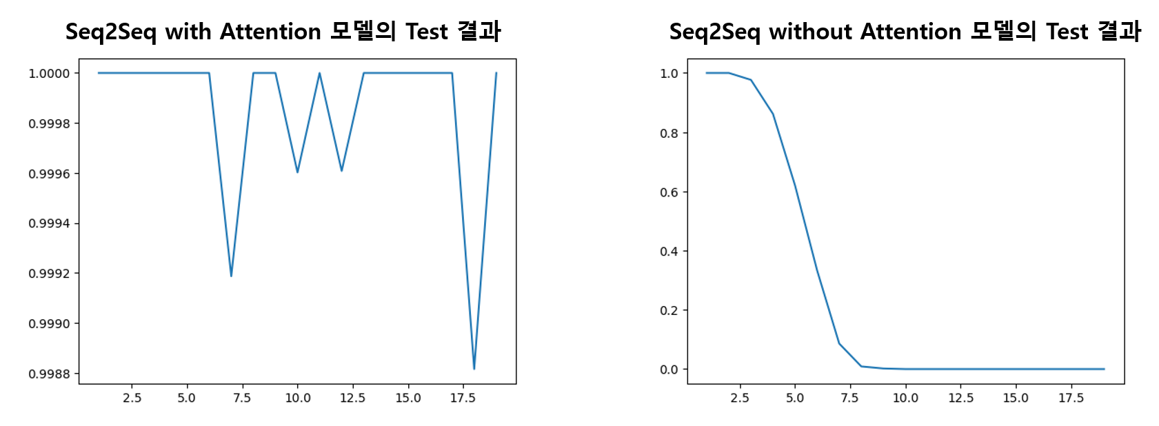 Attention 메커니즘을 적용하지 않은 Seq2Seq 모델에 대해서는 입력되는 Sequence의 길이가 길어질수록 Accuracy가 감소하는 반면, Attention 메커니즘을 적용한 Seq2Seq 모델은 입력 Sequence의 길이가 길어져도 Accuracy 값이 1.0000에서 0.9988 내에서 유지되는 것을 볼 수 있다.
이처럼 Attention 메커니즘을 적용하면 Sequence 길이가 길어질수록 Accuracy가 감소하는 기존 Seq2Seq 모델의 단점을 보완할 수 있다.