Regularization
- 규제를 건다 - 학습을 방해하도록 무엇가를 한다
- why? test 데이터에도 잘 동작할 수 있도록
Early stopping
- 학습을 멈추는 것
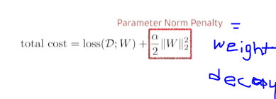
Parameter norm penalty
- 뉴럴네트워크 파라미터를 너무 커지는것을 방지
- 네트워크 파라미터들을 제곱 후 그것을 줄이는것(크기가 작으면 작을수록 좋다)
- 뉴럴 네트워크가 만들어내는 함수의 공간속에서 함수를 최대한 부드러운 함수로 보자
- why? 부드러운 함수일수록 generalization이 좋다
- why? 부드러운 함수일수록 generalization이 좋다
Data augmentation
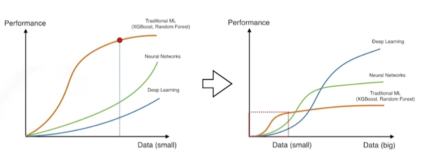
- 데이터가 적으면 딥러닝보다 ML 또는 GD가 더 성과가 잘 나옴
- 데이터가 많아지면 딥러닝이 더 많은 것을 표현할 수 있음
- 데이터가 한정적일 때 Data augmentation을 함

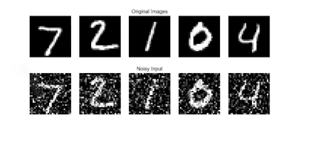
Noise robustness
- 입력 data과 뉴럴네트워크의 weight에 노이즈를 집어넣는것
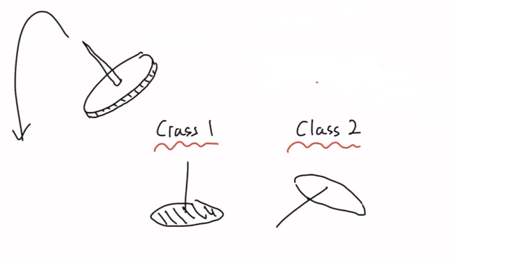
Label smoothing
train 데이터에서 2개를 뽑아서 2개를 섞어줌
- 어떤 효과가 있는가? decision boundary(라벨을 구분하는경계)를 부드럽게 만들어줌!
- Mix-up(섞어줄때 블랜딩하게 2개를 섞음)
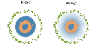
- CutMix(섞어줄때 특정영역으로 구분하여 하나로 만들어줌)
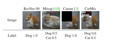
- 노력 대비 성능이 많이 올라감!!
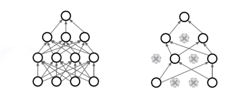
Dropout
뉴럴네트워크의 weight를 0으로 바꿔주는 것 dropout
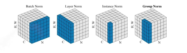
Batch normalization
내가 적용하고자 하는 layer에 statistics를 정교화시키는것
- 각각 뉴럴네트워크의 레이어의 statistics가 Mean zero unit variance 만드는것?
- ex) 100 정도의 값을 가지면 0으로 줄여버림(평균을 빼고 표준편차로 나눠짐)

- ex) 100 정도의 값을 가지면 0으로 줄여버림(평균을 빼고 표준편차로 나눠짐)
- interal 피처 shift를 줄여 학습을 잘 하도록...?
- 이를 다른 논문에서 반박했지만 일반적으로 네트워크가 깊어질수록 성능이 좋아짐
딥러닝 연습
파이토치로 시작하는 딥러닝 기초: Lab-07-2 MNIST Introduction
torchvision
- 파이토치에서 사용하는 패키지: 데이터셋, 모델 아키텍처, 데이터에 적용할수 있는 transforms등을 사용할 수 있음
import torchvision.datasets as dsets
...
# root: 파일의 위치,
# train: True-train set False-test set,
# transform: 데이터를 불러올때 어떤 transform을 사용할 것인가?
## ToTensor: 이미지는 (높이,너비,채널) -> 파이토치의 채널, 높이,너비 순서로 바꿔줌
mnist_train = dsets.MNIST(root="MNIST_data/", train=True, transform=transforms.ToTensor(),
download=True)
mnist_test = dsets.MNIST(root="MNIST_data/", train=False, transform=transforms.ToTensor(),
download=True)

# DataLoader: 어떤 데이터를 로더할꺼냐?
# batch_size: 데이터를 불러올떄 몇개씩 잘라올래?
# shuffle: 무작위를 불러올래? 원래 순서대로 불러올래?
# drop_last: 배치사이즈에 맞게 불러올때 숫자가 맞지 않는 뒷 데이터는 어떻게 할래?(True: 사용하지 않음)
data_loader = torch.utils.DataLoader(DataLoader=mnist_train, batch_size=batch_size,
shuffle=True, drop_last=True)
...
for epoch in range(training_epochs):
...
 for X, Y in data_loader:  # x: 이미지 데이터 Y:label 데이터
 # reshape input image into [batch_size by 784]
 # label is not one-hot encoded
 X = X.view(-1, 28 * 28).to(device)
 ## batch size, 1(크기), 28(높이), 28(너비) -> batch size, 784
Epoch / Batch size / Iteration
- epoch: training set이 한번 돌면 1 epoch가 돌았다.
- Batch size: training set를 얼마나 잘라서 돌릴거냐?(한번에 돌리면 메모리,시간이 부족하다)
- Iteration: 배치를 몇번 학습에 사용했냐?
ex) 1000개 data set-> batch size: 500 -> 2 interation, 1 epoch
Softmax
# MNIST data image of shape 28 * 28 = 784
# 10(output):minist는 10개의 라벨을 사용한다.
linear = torch.nn.Linear(784, 10, bias=True).to(device)

# initialization
torch.nn.init.normal_(linear.weight)

# parameters
training_epochs = 15
batch_size = 100

# define cost/loss & optimizer
criterion = torch.nn.CrossEntropyLoss().to(device) # Softmax is internally computed.

# linear.parameters() -> biase, weight
optimizer = torch.optim.SGD(linear.parameters(), lr=0.1)

for epoch in range(training_epochs):
 avg_cost = 0
 total_batch = len(data_loader)
 for X, Y in data_loader:
 # reshape input image into [batch_size by 784]
 # label is not one-hot encoded
 X = X.view(-1, 28 * 28).to(device)
 optimier.zero_grad()
 hypothesis = linear(X)  # 분류결과를 얻을 수 있음
 cost = criterion(hypothesis, Y) # 분류결과와 정답 라벨을 CrossEntropy을 구해서 cost 구함
 cost.backward() # 그래디언트를 계산
 optimizer.step() # 업데이트 진행
 avg_cost += cost / total_batch
 print("Epoch: ", "%04d" % (epoch+1), "cost =", "{:.9f}".format(avg_cost))
test
# Test the model using test sets
With torch.no_grad():  #grad 계산하지 않겠다
 X_test = mnist_test.test_data.view(-1, 28 * 28).float().to(device)
 Y_test = mnist_test.test_labels.to(device)

 prediction = linear(X_test) # 예측한 결과를 받음
 correct_prediction = torch.argmax(prediction, 1) == Y_test # 정답 테이블과 예측값이 일치하냐?
 accuracy = correct_prediction.float().mean()
 print("Accuracy: ", accuracy.item())
Visualization
- 실제 예측한 값을 이미지로 볼 수 있도록 함
import matplotlib.pyplot as plt
import random
...
r = random.randint(0, len(mnist_test) - 1)
X_single_data = mnist_test.test_data[r:r + 1].view(-1, 28 *28).float().to(device)
Y_single_data = mnist_test.test_labels[r:r + 1].to(device)

print("Label: ", Y_single_data.item())
single_prediction = linear(X_single_data)
print("Prediction: ", torch.argmax(single_prediction,
1).item())

# 예측을 해본 이미지를 띄운다
plt.imshow(mnist_test.test_data[r:r + 1].view(28, 28),
cmap="Greys", interpolation="nearest")
plt.show()
파이토치로 시작하는 딥러닝 기초: Lab-07-1 Tips
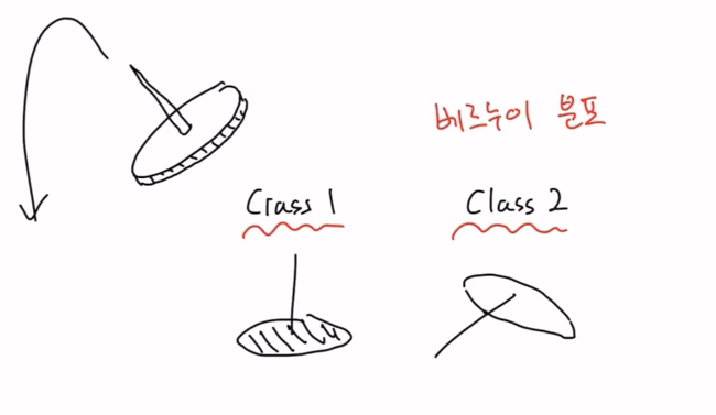
최대 가능도 추정(Maximum Likelihood Estimation)
예를 들어 압정을 던졌을 때, 바닥으로 떨어질지? 아님 압정 뾰족한 부분으로 떨어질지?
- 베루누이 분포를 이용
- binary distributaion 공식
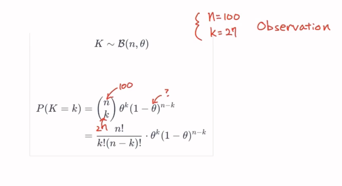
- 우리가 알고싶은건 θ임
- θ: 압정의 확률분포를 결정하는 파라미터
- 뉴럴네트워크가 될 수도 있고,베르누이 또는 binary distributaion에서 결정하는 θ값일 수 있음
- 위 공식을 그래프로 표현
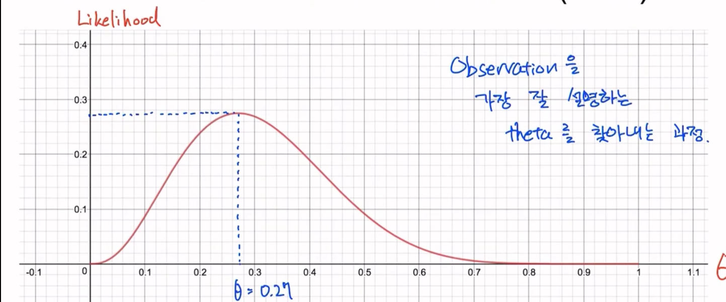
- 그렇다면 그래프에서 최대가 되는걸 어떻게 구함? 기울기 구하면 됨!
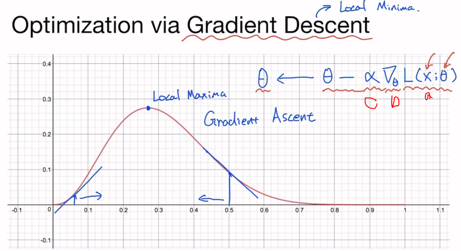
- a: 손실함수에 데이터x와 θ 넣은 것
- b: θ에 대해 미분
- c: learning rate
과적합(Overfitting)과 정규화(Regurlarization)
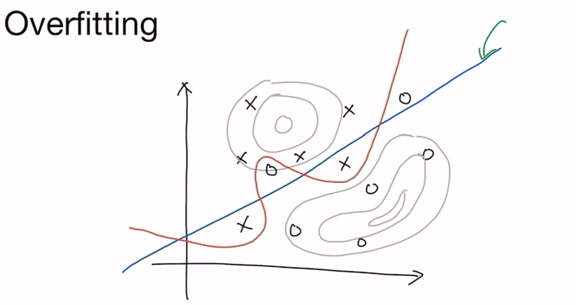
그렇다면 어떻게 Overfitting을 방지할 수 있을까?
- 전체 observation을 훈련 set(0,8)과 Dev set(0.1), test set(0.1~0.2)으로 나눠서 사용
- Dev set = Validation set
- Dev set = Validation set
- More Data
- Less features
- Regurlarization
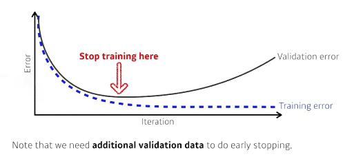
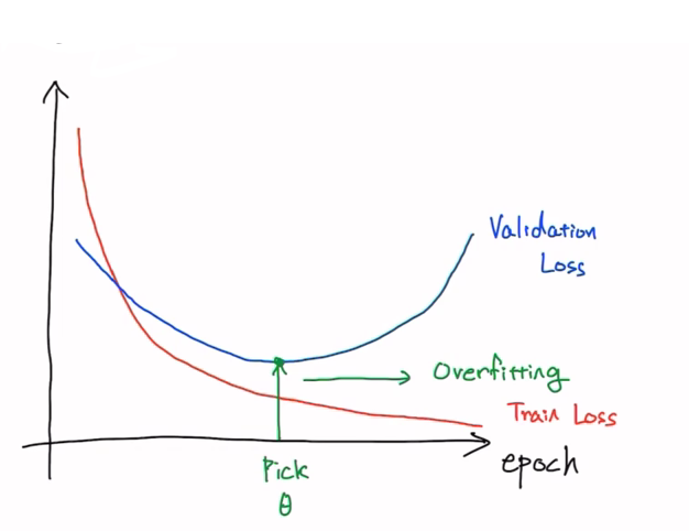
- Early Stopping: validation Loss가 더 이상 낮아지지 않을때 stop
- Reducing Network Size
- Weight Decay: 뉴럴네트워크의 파라미터 크기를 제한
- Dropout(많이 쓰임)
- Batch Normalization(많이 쓰임)
Training and Test Dataset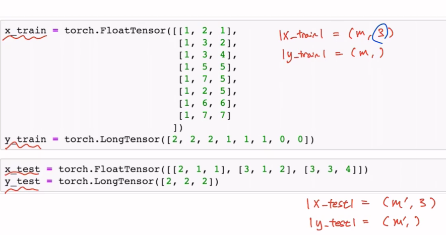
Model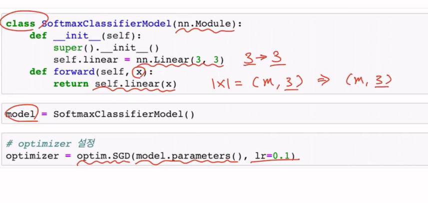
Training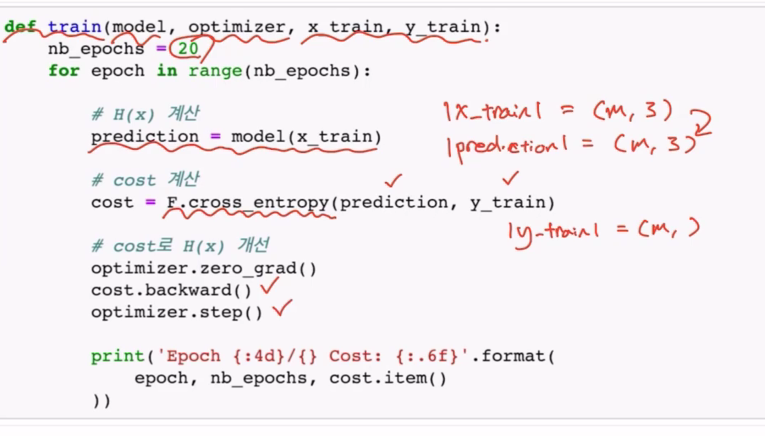
test(Validation)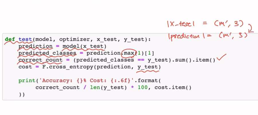
Runing 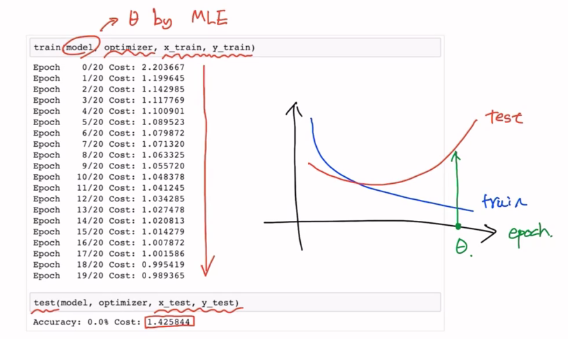
Data Preprocessing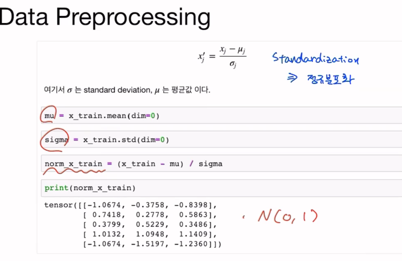
Training with Preprocessed Data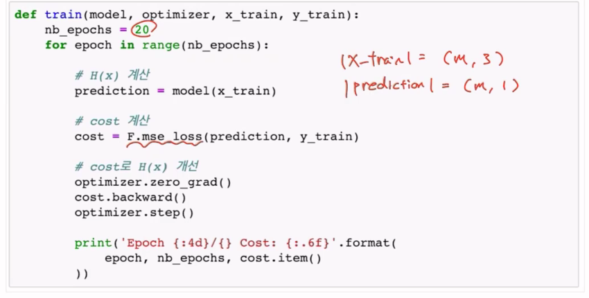
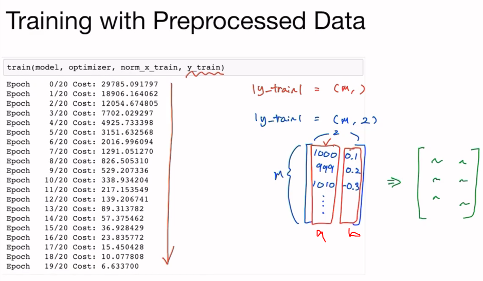
- 만일 전처리를 하지 않았더라면 a 데이터만 신경쓰고 b는 신경쓰지 않았을 것 그러므로 전처리로 비슷하게 만들어줌
파이토치로 시작하는 딥러닝 기초: Lab-08-2 Multi Layer Perceptron
XOR
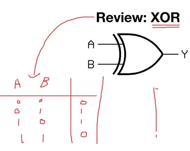
- XOR는 단층 퍼셉트론으로는 해결할 수 없음
Multi Layer Perceptron
- XOR를 해결하기 위해서는 Multi Layer Perceptron이 필요하다
- 한개 이상의 층을 가진 Perceptron
- 한개 이상의 층을 가진 Perceptron
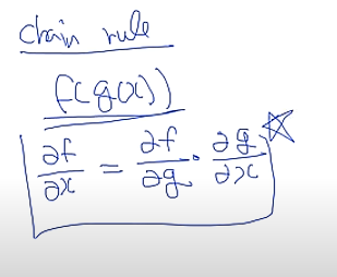
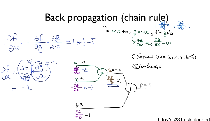
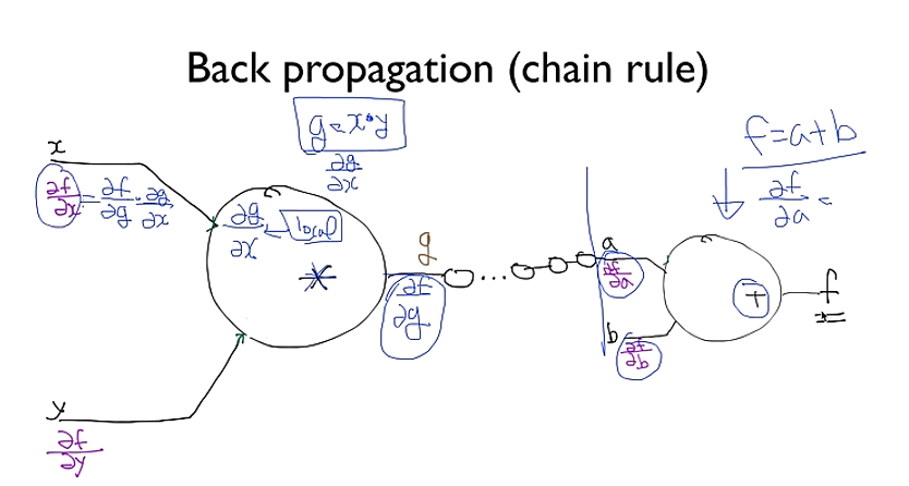
Backpropagation
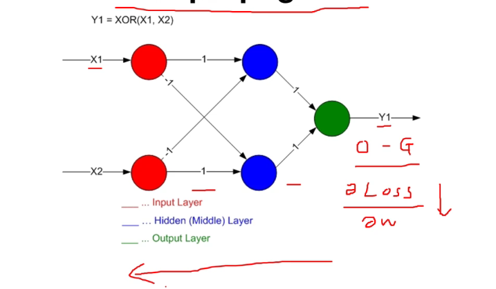
- [참고]모두를 위한 딥러닝 강좌1 - Backpropagation
X = torch.FloatTensor([[0, 0], [0, 1], [1, 0], [1, 1]]).to(device)
Y = torch.FloatTensor([[0], [1], [1], [0]]).to(device)
# nn layers => nn.linear 2개를 사용했다
w1 = torch.Tensor(2, 2).to(device)
b1 = torch.Tensor(2).to(device)
w2 = torch.Tensor(2, 1).to(device)
b2 = torch.Tensor(1).to(device)
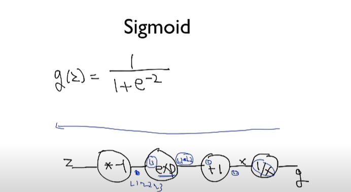
def sigmoid(x):
# sigmoid function
return 1.0 / (1.0 + torch.exp(-x))
# return torch.div(torch.tensor(1), torch.add(torch.tensor(1.0), torch.exp(-x)))
def sigmoid_prime(x): # 시그모이드 미분
# derivative of the sigmoid function
return sigmoid(x) * (1 - sigmoid(x))for step in range(10001):
# forward
l1 = torch.add(torch.matmul(X, w1), b1)
a1 = sigmoid(l1)
l2 = torch.add(torch.matmul(a1, w2), b2)
Y_pred = sigmoid(l2)
#binary cross Entropy
cost = -torch.mean(Y * torch.log(Y_pred) + (1 - Y) * torch.log(1 - Y_pred))for step in range(10001):
# forward
...
# Back prop (chain rule)
# Loss( #binary cross Entropy) derivative
# 1e-7 -> 0으로 나눠지는 것을 방지하기 위해서
d_Y_pred = (Y_pred - Y) / (Y_pred * (1.0 - Y_pred) + 1e-7)
# Layer 2
d_l2 = d_Y_pred * sigmoid_prime(l2) # 시그모이드에 대한 미분 사용
d_b2 = d_l2 # bias에 대한 미분
# matmul: 매트릭스 곱
# transpose -> matrix의 transpose와 비슷 ex) 10 X 5 -> 5 X 10
d_w2 = torch.matmul(torch.transpose(a1, 0, 1), d_b2) # weight에 대한 미분
# Layer 1
d_a1 = torch.matmul(d_b2, torch.transpose(w2, 0, 1))
d_l1 = d_a1 * sigmoid_prime(l1)
d_b1 = d_l1
d_w1 = torch.matmul(torch.transpose(X, 0, 1), d_b1)for step in range(10001):
# forward
...
# Back prop (chain rule)
...
# Weight update
w1 = w1 - learning_rate * d_w1
b1 = b1 - learning_rate * torch.mean(d_b1, 0)
w2 = w2 - learning_rate * d_w2
b2 = b2 - learning_rate * torch.mean(d_b2, 0)
if step % 100 == 0:
print(step, cost.item())
Code: xor-nn
X = torch.FloatTensor([[0, 0], [0, 1], [1, 0], [1, 1]]).to(device)
Y = torch.FloatTensor([[0], [1], [1], [0]]).to(device)

# nn layers (Multi Layer Perceptron)
linear1 = torch.nn.Linear(2, 2, bias=True)
linear2 = torch.nn.Linear(2, 1, bias=True)
sigmoid = torch.nn.Sigmoid()
model = torch.nn.Sequential(linear1, sigmoid, linear2, sigmoid).to(device)

# define cost/loss & optimizer
criterion = torch.nn.BCELoss().to(device)
optimizer = torch.optim.SGD(model.parameters(), lr=1)

for step in range(10001):
 optimizer.zero_grad()
 hypothesis = model(X)
 # cost/loss function
 cost = criterion(hypothesis, Y)
 cost.backward()
 optimizer.step()
 if step % 100 == 0:
 print(step, cost.item())
Code: xor-nn-wide-deep
X = torch.FloatTensor([[0, 0], [0, 1], [1, 0], [1, 1]]).to(device)
Y = torch.FloatTensor([[0], [1], [1], [0]]).to(device)

# nn layers
linear1 = torch.nn.Linear(2, 10, bias=True)
linear2 = torch.nn.Linear(10, 10, bias=True)
linear3 = torch.nn.Linear(10, 10, bias=True)
linear4 = torch.nn.Linear(10, 1, bias=True)
sigmoid = torch.nn.Sigmoid()
마루에 미친자