DAY33

특성 중요도

Feature Importances(Mean decrease impurity, MDI)

• sklearn 트리 기반 분류기에서 디폴트로 사용
• 속도는 빠르지만 결과를 주의해서 봐야함
  • Warning: impurity-based feature importances can be misleading for high cardinality features (many unique values)
  • high cardinality features-> 과적합될 위험 有
• 각각 특성을 모든 트리에 대해 평균불순도감소(mean decrease impurity)를 계산한 값
• DAY27

rf = pipe.named_steps['randomforestclassifier']
importances = pd.Series(rf.feature_importances_, X_train.columns)

# 시각화
%matplotlib inline
import matplotlib.pyplot as plt

n = 20
plt.figure(figsize=(10,n/2))
plt.title(f'Top {n} features')
importances.sort_values()[-n:].plot.barh();

Drop-Column Importance

• 매 특성을 drop한 후 fit
• 이론적으로 가장 좋아보이지만 손으로 하나하나 하는 것이기 때문에 매우 느림
• 예시는 N233

순열중요도(Permutation Importance, Mean Decrease Accuracy,MDA)

• 기본 특성 중요도와 Drop-column 중요도 중간에 위치
• 관심있는 특성에만 무작위로 노이즈를 주고 예측을 하였을 때 성능 평가지표(정확도, F1, R2 등)가 얼마나 감소하는지를 측정
  • 검증데이터에서 각 특성을 제거하지 않고 특성값에 무작위로 노이즈를 주어 기존 정보를 제거하여 특성이 기존에 하던 역할을 하지 못하게 하고 성능을 측정
    • 노이즈를 준다는 것은 기존의 정보를 제거하거나 제 기능을 하지 못하게 하는 것
  • 노이즈를 주는 가장 간단한 방법이 그 특성값들을 샘플들 내에서 섞는 것(shuffle, permutation)
• 재학습이 필요없음
• high cardinality features 중요도 부풀려지는 걸 바로 잡을 수 있음

---

eli5 라이브러리

pipe 라인 생성

from sklearn.pipeline import Pipeline
from sklearn.pipeline import make_pipeline
pipe = Pipeline([
    ('preprocessing', make_pipeline(OrdinalEncoder(), SimpleImputer())),
    ('rf', RandomForestClassifier(n_estimators=100, random_state=2, n_jobs=-1)) 
])
pipe.fit(X_train, y_train)

import warnings 
warnings.simplefilter(action='ignore', category=FutureWarning)

import eli5
from eli5.sklearn import PermutationImportance

# permuter 정의
permuter = PermutationImportance(
    pipe.named_steps['rf'], # model
    scoring='accuracy', # metric
    n_iter=5, # 다른 random seed를 사용하여 5번 반복
    random_state=2
)

# permuter 계산은 preprocessing 된 X_val을 사용합니다.
X_val_transformed = pipe.named_steps['preprocessing'].transform(X_val)

# 실제로 fit 의미보다는 스코어를 다시 계산하는 작업입니다
permuter.fit(X_val_transformed, y_val);

특성별 Score 확인

eli5.show_weights(
    permuter, 
    top=None, # top n 지정 가능, None 일 경우 모든 특성 
    feature_names=feature_names # list 형식으로 넣어야 합니다
)

중요도를 이용하여 특성을 선택

minimum_importance = 0.001

mask = permuter.feature_importances_ > minimum_importance
features = X_train.columns[mask]
X_train_selected = X_train[features]
X_val_selected = X_val[features]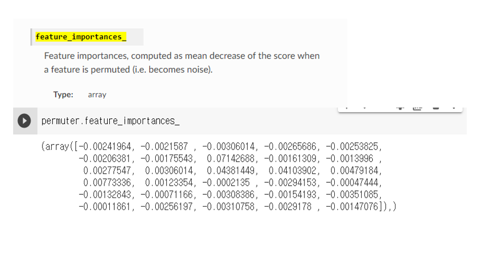

공식문서

Boosting(xgboost for gradient boosting)

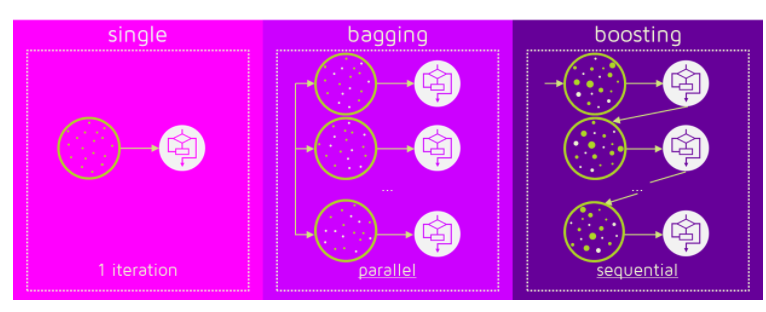
• 배깅이나 부스팅 앙상블 모델을 사용해 과적합을 피함
• 랜덤포레스트의 장점은 하이퍼파라미터에 상대적으로 덜 민감하나 그래디언트 부스팅의 경우, 하이퍼파라미터 셋팅에 따라 더 좋은 예측 성능을 보여줌

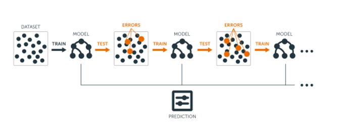
부스팅 vs 배깅

• 배깅에는 랜덤포레스트 모델이, 부스팅에는 AdaBoost와 gradient boosting이 대표적인 모델임
• 랜덤포레스트의 경우 각 트리를 독립적으로 만들지만, 부스팅은 만들어지는 트리가 이전에 만들어진 트리에 영향을 받음
  이미지 출처

AdaBoost의 알고리즘

• 각 트리(weak learners)가 만들어질 때 잘못 분류되는 관측치에 가중치를 줍다
  • 가중치를 준다는 것은 샘플링에서 더 잘 뽑힐 확률이라고 생각
• 그 다음 트리를 만들때 이전에 절못 분류된 관측치가 더 많이 샘플링되게 하여 그 관측치를 분류하는데 더 초점을 맞춘다.

---

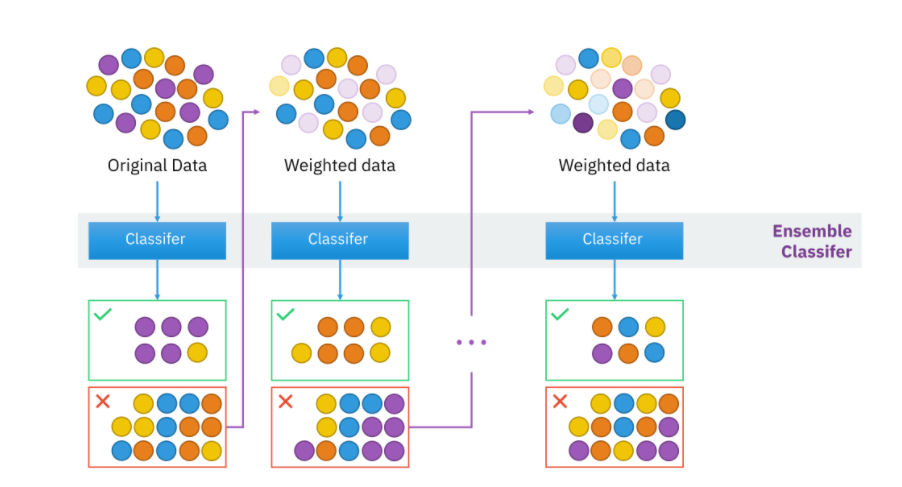
Step 0. 모든 관측치에 대해 가중치를 동일하게 설정 합니다.

Step 1. 관측치를 복원추출 하여 약한 학습기 Dn을 학습하고 +, - 분류 합니다.

Step 2. 잘못 분류된 관측치에 가중치를 부여해 다음 과정에서 샘플링이 잘되도록 합니다.

Step 3. Step 1~2 과정을 n회 반복(n = 3) 합니다.

Step 4. 분류기들(D1, D2, D3)을 결합하여 최종 예측을 수행합니다.

---

gradient boosting

• 회귀와 분류문제에 모두 사용
• AdaBoost와 유사하지만 비용함수(Loss function)을 최적화하는 방법
  • 샘플의 가중치를 조정하는 대신 잔차을 학습
    • 잔차가 더 큰 데이터를 더 학습하도록 만드는 효과 有
• Python libraries for Gradient Boosting:
  scikit-learn Gradient Tree Boosting, xgboost, LightGBM, CatBoost

XGBoost Python API Reference: Scikit-Learn API

from xgboost import XGBClassifier
pipe = make_pipeline(
    OrdinalEncoder(),
    SimpleImputer(strategy='median'),
    XGBClassifier(n_estimators=200
                  , random_state=2
                  , n_jobs=-1
                  , max_depth=7
                  , learning_rate=0.2
                 )
)
pipe.fit(X_train, y_train);

---

Early Stopping

• n_estimators 최적화를 위해 GridSearchCV나 반복문 대신 early stopping을 사용
  • 더이상 모델 성능이 높아지지 않으면 거기서 stop함으로써 과적합 방지와 시간 비용 감소
  • 불필요한 실행의 연속 방지
• early stopping을 사용하면 우리는 n_iterations 만큼의 트리를 학습
  • GridSearchCV나 반복문을 사용하면 많은 실행 하게 됨
    

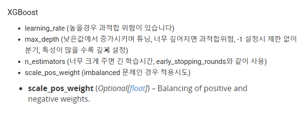
model = XGBClassifier(
    n_estimators=1000,  # <= 1000 트리로 설정했지만, early stopping 에 따라 조절됩니다.
    max_depth=7,        # default=3, high cardinality 특성을 위해 기본보다 높여 보았습니다.
    learning_rate=0.2,
#     scale_pos_weight=ratio, # imbalance 데이터 일 경우 비율을 적용합니다.
    n_jobs=-1
)

eval_set = [(X_train_encoded, y_train), 
            (X_val_encoded, y_val)]

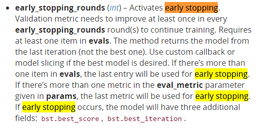
model.fit(X_train_encoded, y_train, 
          eval_set=eval_set,
          eval_metric='error', # #(wrong cases)/#(all cases)
          early_stopping_rounds=50
         ) # 50 rounds 동안 스코어의 개선이 없으면 멈춤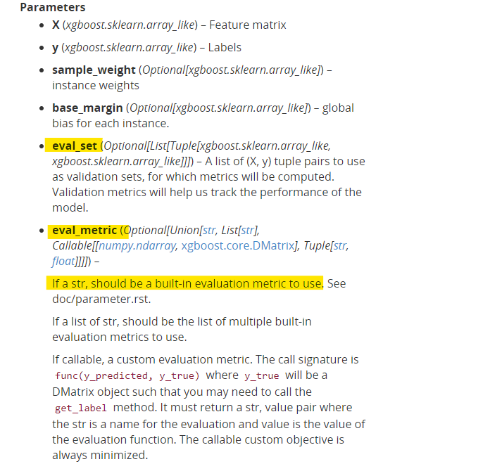

공식문서

N233

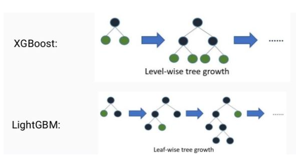
LightGBM

[배경]

• Xgboost는 학습시간이 느리다는 단점이 있으며, 하이퍼파라미터도 많음
  • 그리드 서치같이 하이퍼파라미터를 튜닝하게 되면 더욱 시간이 오래 걸림
• 위와 같은 단점을 보완하여 나온것이 LightGBM임

[장점]

• 대용량데이터 처리가 가능
• 더 적은 자원을 사용하며 빠르다
• GPU까지 지원

[특징]

• leaf wise(리프 중심)트리분할을 사용
  • 트리의 균형을 맞추지 않고 리프 노드를 지속적으로 분할 진행
    • level-wise 방식은 트리의 균형을 잡아주어야 하기 때문에 deth 줄어듬
  • max delta loss 값을 가지는 피트 노드를 계속 분할 하기 대문에 비대칭적이고 깊은 트리가 생성되지만 level-wise보다 손실을 줄일 수 있다

from lightgbm import  LGBMClassifier

pipe3 = make_pipeline(
    OrdinalEncoder(),
    SimpleImputer(strategy='median'),
    LGBMClassifier(n_estimators=200
                  , random_state=2
                  , n_jobs=-1
                  , max_depth=7
                  , learning_rate=0.2
                 )
)

pipe3.fit(X_train, y_train);

출처

더 알아야할 것

eval_metric= 에 들어갈 수 있는 평가 지표들 알아보기