Image Classification
tf.data.Dataset을 이용해 모델이 데이터를 효율적으로 활용할 수 있도록 구현해보는게 목적입니다.
기본적인 머신러닝 작업과정은 아래와 같습니다.
- Examine and understand data
- Build an input pipeline
- Build the model
- Train the model
- Test the model
- Improve the model and repeat the process
모델 완성 후 평가 지표에 따라서 모델을 평가해 봅시다.
Project 설명
Task
- CIFAR 10 데이터셋을 이용해 classification을 진행해보자.
- CIFAR 10 Dataset
Baseline
-
오버피팅을 방지하기 위한 다양한 방법들을 사용해보자.
- 하이퍼파라미터 조절 (데이터 로드, 모델, Optimizer 등)
- 모델 구성 변경 (layer의 갯수)
-
Training
- tf.data.Dataset 과 model.fit()을 사용
-
Evaluation
- 모델의 정확도와 크기를 이용해 점수를 제공하는 메트릭으로 평가해보자.
구글 드라이브 마운트
- Google의 Colab과 Drive를 이용해 노트북을 이용해 언제 어디서든 딥러닝 모델을 학습시켜보자.
# 코드 호환성을 위한 분기
use_colab = True
assert use_colab in [True, False]
from google.colab import drive
drive.mount('/content/drive')Drive already mounted at /content/drive; to attempt to forcibly remount, call drive.mount("/content/drive", force_remount=True).번외) GPU 서버를 어떻게 구성하면 좋을까?
-
로컬 머신 (노트북, 데스크탑) 구매
- GPU 노트북, 데스크탑, 서버 등 원하는 방법으로 다양하게 구비할 수 있다.
- Colab과 다르게 세션이 종료되지않으며, 비교적 자유롭게 사용할 수 있다.
- 원격 접속 및 오프라인 관리가 어려우며, 부수적인 유지보수 비용이 발생한다.
클라우드 등 서버 사용
-
AWS, 네이버 클라우드 등
- 오프라인 관리가 필요없으며, 안정적이다.
- 비싸다...
import packages
import tensorflow as tf
from tensorflow.keras.models import Sequential
from tensorflow.keras import layers

from sklearn.model_selection import train_test_split

import numpy as np
import matplotlib.pyplot as plt
import os

tf.__version__
load data
- CIFAR 10 dataset을 로드한다. (npy)
- 학습에 사용되는 대표적인 데이터셋들은 프레임워크내 코드로 제공된다.
tf.keras.dataset.cifar10
tf.keras.dataset.cifar100
tf.keras.dataset.mnist
tf.keras.dataset.fashion_mnist
tf.keras.dataset.imdb
- 다양한 데이터셋을 쉽게 가져와 사용할 수 있다.
데이터셋 사용방법
- Data split
- sklearn (머신러닝 프레임워크)를 이용해 데이터를 손쉽게 나눌 수 있다.
test_data_split, valid_data, test_labels_split, valid_labels = \
    train_test_split(test_data, test_labels, test_size=0.2, shuffle=True)
- test_size를 조절해 원하는 크기만큼의 데이터를 분리해 사용할 수 있다.
# Load training and eval data from tf.keras
(train_data, train_labels), (test_data, test_labels) = \
    tf.keras.datasets.cifar10.load_data()
!cd /root/.keras/datasets/ && ls -al#total 166520
#drwxr-xr-x 3 root root 4096 Dec 29 01:11 .
#drwxr-xr-x 1 root root 4096 Dec 29 01:11 ..
#drwxr-xr-x 2 2156 1103 4096 Jun 4 2009 cifar-10-batches-py
#-rw-r--r-- 1 root root 170498071 Dec 29 01:11 cifar-10-batches-#py.tar.gzprint(train_data.shape, train_labels.shape)
print(test_data.shape, test_labels.shape)
print(test_labels[0]) # 데이터셋 제작할때, [3] => 3 으로 데이터 형태를 변경해줘야합니다.#(50000, 32, 32, 3) (50000, 1)
#(10000, 32, 32, 3) (10000, 1)
#[3]test_data, valid_data, test_labels, valid_labels = \
train_test_split(test_data, test_labels, test_size=0.1, shuffle=True) # 0~1의 값으로 줍니다.
# test_size => 0.1 = 10%
# test_size => 0.2 = 20%
# raw data normalization
# RGB 값이 0~255 사이 값인 것을 이용해 Normalization 진행
train_data = train_data / 255.
train_data = train_data.reshape([-1, 32, 32, 3])
train_labels = train_labels.reshape([-1]) #
valid_data = valid_data / 255.
valid_data = valid_data.reshape([-1, 32, 32, 3])
valid_labels = valid_labels.reshape([-1])
test_data = test_data / 255.
test_data = test_data.reshape([-1, 32, 32, 3])
test_labels = test_labels.reshape([-1])# [데이터수, 32, 32, 3] [데이터수,]
print(train_data.shape, train_labels.shape)
print(valid_data.shape, valid_labels.shape)
print(test_data.shape, test_labels.shape)#(50000, 32, 32, 3) (50000,)
#(1000, 32, 32, 3) (1000,)
#(9000, 32, 32, 3) (9000,)dataset 구성
- tf.data.Dataset을 이용해 데이터셋을 구성한다
- 위에서 불러온 raw data (cifar10) 데이터셋을 모델이 학습 할 수 있도록 전달해 주는 데이터셋이다.
- tf data Dataset을 사용해야하는 이유?
- 직접 Generator를 작성할 필요가 없다
- map 함수를 이용해 전처리 과정을 직접 조절할 수 있다.
- 메모리에 부담이 되지 않게 동작한다.
직접 적용해보자
- map 함수를 적용할 함수 구현 후 dataset을 구현하며 사용해보자
def one_hot_label(image, label): # label => one_hot
  label = tf.one_hot(label, depth=10)
return image, label- 위 one_hot_label 함수는 아래와 같이 동작한다
one_hot vector 예시
tf.one_hot(
    indices, depth, on_value=None, off_value=None, axis=None, dtype=None, name=None
)
#
indices = [0, 1, 2]
depth = 3
tf.one_hot(indices, depth)  # output: [3 x 3]
# [[1., 0., 0.],
#  [0., 1., 0.],
#  [0., 0., 1.]]
map 함수를 포함한 dataset 구성
- Dataset을 딥러닝 데이터를 쉽게 불러오기 위한 일종의 Generator 입니다.
- 학습에 사용할 데이터셋은 총 3개
- Train dataset, Valid dataset, Test dataset 입니다.
- Raw data에서 분리한 데이터들
- Train dataset, Valid dataset, Test dataset 입니다.
- 데이터셋은 tf.data.Dataset으로 구성되며, 구현 파트에선 데이터를 불러오는 형식만을 지정해준다.
- shuffle, batch 옵션을 이용해 다양하게 데이터를 로드해올 수 있다.
batch_size = 32# for train
N = len(train_data)
train_dataset = tf.data.Dataset.from_tensor_slices((train_data, train_labels))
train_dataset = train_dataset.map(one_hot_label) # 함수의 이름을 써서 구현
train_dataset = train_dataset.shuffle(10000).repeat().batch(batch_size=batch_size)
print(train_dataset)
# # for valid
valid_dataset = tf.data.Dataset.from_tensor_slices((valid_data, valid_labels))
valid_dataset = valid_dataset.map(one_hot_label)
valid_dataset = valid_dataset.batch(batch_size=batch_size)
print(valid_dataset)
# # for test
test_dataset = tf.data.Dataset.from_tensor_slices((test_data, test_labels))
test_dataset = test_dataset.map(one_hot_label)
test_dataset = test_dataset.batch(batch_size=batch_size)
print(test_dataset)#<_BatchDataset element_spec=(TensorSpec(shape=(None, 32, 32, 3), dtype=tf.float64, name=None), TensorSpec(shape=(None, 10), dtype=tf.float32, name=None))>
#<_BatchDataset element_spec=(TensorSpec(shape=(None, 32, 32, 3), dtype=tf.float64, name=None), TensorSpec(shape=(None, 10), dtype=tf.float32, name=None))>
#<_BatchDataset element_spec=(TensorSpec(shape=(None, 32, 32, 3), dtype=tf.float64, name=None), TensorSpec(shape=(None, 10), dtype=tf.float32, name=None))>- 데이터 타입의 경우 Tensorflow 버전에 따라 tf.float32 or tf.float64로 출력될 수 있으나 학습에 큰 영향을 주진 않는다.
- 해당 자료형은 tf.cast를 이용해 따로 타입을 지정해줄 수 있다.
Save point 설정
- Model weight를 저장할 폴더를 지정한다.
- 폴더가 없다면 새로 생성해준다.
# the save point
if use_colab:
    checkpoint_dir ='./drive/My Drive/train_ckpt/cifar10_classification/exp1'
else:
    checkpoint_dir = 'cifar10_classification/exp1'

if not os.path.isdir(checkpoint_dir):
    os.makedirs(checkpoint_dir)
Model Savepoints
- 모델 저장시 모델의 파라미터를 저장한다.
- 위에 구현된 모델의 shape을 기준으로 파라미터만 저장
- 저장된 데이터는 checkpoint 형태로 저장되며, load data를 이용해 불러올 수 있다.
- 저장된 모델 데이터를 불러올 시에는 저장된 모델과 같은 shape인 모델이 메모리 상에 있어야 한다.
model = model() # 구현했던 모델
model.load_weights(checkpoint_dir)
데이터 확인
- 학습에 사용할 데이터를 확인해보자.
index = 219 # index를 변경해 확인해보자 (0~49999)
print("label = {}".format(train_labels[index]))
plt.imshow(train_data[index].reshape(32, 32, 3))
plt.colorbar()
#plt.gca().grid(False)
plt.show()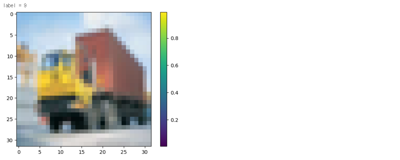
모델 구성
- 직접 모델을 구현해 본다.
class Conv(tf.keras.Model):
    def __init__(self, num_filters, kernel_size=3):
        super(Conv, self).__init__() # 재료창고, 자제창고
        self.conv1 = layers.Conv2D(num_filters, kernel_size, padding='same')
        self.conv2 = layers.Conv2D(num_filters, kernel_size, padding='same')
        self.bn1 = layers.BatchNormalization()
        self.bn2 = layers.BatchNormalization()

    def call(self, inputs, skip=None, training=True):
        x = self.conv1(inputs)
        x = self.bn1(x)
        x = layers.Activation('relu')(x)
        x = self.conv2(x)
        x = self.bn2(x)
        if skip is not None:
            x = tf.concat([x, inputs], -1)
        x = layers.Activation('relu')(x)

        return x


class Dense(tf.keras.Model):
    def __init__(self, num_nodes=1024):
        super(Dense, self).__init__()
        self.dense1 = layers.Dense(num_nodes)
        self.dense2 = layers.Dense(num_nodes)
        self.bn1 = layers.BatchNormalization()
        self.bn2 = layers.BatchNormalization()

    def call(self, inputs, training=True):
        x = self.dense1(inputs)
        x = self.bn1(x)
        x = layers.Activation("relu")(x)
        x = layers.Dropout(0.5)(x)
        x = self.dense2(x)
        x = self.bn2(x)
        x = layers.Activation("relu")(x)

        return x

class VGGlikeModel(tf.keras.Model):
    def __init__(self):
        super(VGGlikeModel, self).__init__()
        self.conv_block1 = Conv(32)
        self.conv_block2 = Conv(64)
        self.conv_block3 = Conv(128)
        self.conv_block4 = Conv(256)
        self.fc = Dense()
        self.outputs = layers.Dense(10)

    def call(self, inputs, training=True):
        x = self.conv_block1(inputs, True)
        x = layers.MaxPooling2D()(x)
        x = self.conv_block2(x, True)
        x = layers.MaxPooling2D()(x)
        x = self.conv_block3(x, True)
        x = layers.MaxPooling2D()(x)
        x = self.conv_block4(x, True)
        x = layers.Flatten()(x)
        x = self.fc(x)
        x = self.outputs(x)

        return x

model = VGGlikeModel()
# input_tensor = layers.Input(shape=(32, 32, 3,))
# x = layers.Conv2D(32, 3, padding='same',
# kernel_initializer=tf.keras.initializers.HeUniform())(input_tensor)
# x = layers.BatchNormalization()(x)
# x = layers.Activation('relu')(x)
# x = layers.Conv2D(32, 3, padding='same',
# kernel_initializer=tf.keras.initializers.HeUniform())(input_tensor)
# x = layers.BatchNormalization()(x)
# x = layers.Activation('relu')(x)
# x_skip = layers.MaxPooling2D()(x) # 16, 16, 32
# x = layers.Conv2D(64, 3, padding='same',
# kernel_initializer=tf.keras.initializers.HeUniform())(x_skip)
# x = layers.BatchNormalization()(x)
# x = layers.Activation('relu')(x)
# x = layers.Conv2D(64, 3, padding='same',
# kernel_initializer=tf.keras.initializers.HeUniform())(x)
# x = layers.BatchNormalization()(x)
# x = layers.Activation('relu')(x)
# x = layers.Conv2D(64, 3, padding='same',
# kernel_initializer=tf.keras.initializers.HeUniform())(x)
# x = layers.BatchNormalization()(x) # 16, 16, 64
# x = tf.concat([x, x_skip], -1) # 16, 16, 96
# x = layers.Activation('relu')(x)
# x = layers.MaxPooling2D()(x)
# x = layers.Conv2D(128, 3, padding='same',
# kernel_initializer=tf.keras.initializers.HeUniform())(x)
# x = layers.BatchNormalization()(x)
# x = layers.Activation('relu')(x)
# x = layers.Conv2D(128, 3, padding='same',
# kernel_initializer=tf.keras.initializers.HeUniform())(x)
# x = layers.BatchNormalization()(x)
# x = layers.Activation('relu')(x)
# x = layers.Conv2D(128, 3, padding='same',
# kernel_initializer=tf.keras.initializers.HeUniform())(x)
# x = layers.BatchNormalization()(x)
# x = layers.Activation('relu')(x)
# x = layers.MaxPooling2D()(x)
# x = layers.Conv2D(256, 3, padding='same',
# kernel_initializer=tf.keras.initializers.HeUniform())(x)
# x = layers.BatchNormalization()(x)
# x = layers.Activation('relu')(x)
# x = layers.Conv2D(256, 3, padding='same',
# kernel_initializer=tf.keras.initializers.HeUniform())(x)
# x = layers.BatchNormalization()(x)
# x = layers.Activation('relu')(x)
# x = layers.Conv2D(256, 3, padding='same',
# kernel_initializer=tf.keras.initializers.HeUniform())(x)
# x = layers.BatchNormalization()(x)
# x = layers.Activation('relu')(x)
# x = layers.Flatten()(x)
# x = layers.Dense(1024,
# kernel_initializer=tf.keras.initializers.HeUniform())(x)
# x = layers.BatchNormalization()(x)
# x = layers.Activation('relu')(x)
# x = layers.Dropout(0.5)(x)
# x = layers.Dense(1024,
# kernel_initializer=tf.keras.initializers.HeUniform())(x)
# x = layers.BatchNormalization()(x)
# x = layers.Activation('relu')(x)
# output_tensor = layers.Dense(10)(x)
# model = tf.keras.Model(input_tensor, output_tensor)- 모델이 잘 생성 되었는지 간단하게 테스트해 봅시다.
# without training, just inference a model in eager execution:
predictions = model(train_data[0:1], training=False)
print("Predictions: ", predictions.numpy()) # 총 10개의 데이터가 나오면 모델이 잘 구성된겁니다.
#Predictions: [[ 0.01264782 0.03612096 0.06472357 0.18101807 0.05038511 0.01011162
# -0.13988994 0.00797083 -0.1587979 -0.04783075]]- 위 Predictions 결과가 총 10개 짜리 리스트로 출력 된다면, 현재 테스크에서 정상적인 출력입니다.
- cifar10 dataset은 정답이 총 10개로 이뤄져 있습니다.
- 출력값은 마지막 output layer에 activation의 유무에 따라서 값이 달라지며, activation을 통과하기전 데이터를 logit이라고 이야기합니다.
Model compile
- 학습을 위한 Optimizer와 Loss fn을 설정해준다.
- Optimzier는 learning rate를 인자로 가지며, 모델의 학습정도를 컨트롤합니다.
- Loss fn은 모델의 예측결과와 실제 정답간의 차이를 loss로 계산해 모델을 학습합니다.
model.compile(optimizer=tf.keras.optimizers.Adam(), # learning rate가 기본값으로 1e-3으로 들어가있습니다.
              loss=tf.keras.losses.CategoricalCrossentropy(from_logits=True),
metrics=['accuracy'])model.summary()Model: "vg_glike_model"
_________________________________________________________________
Layer (type) Output Shape Param #
=================================================================
conv (Conv) multiple 10400
conv_1 (Conv) multiple 57664
conv_2 (Conv) multiple 262784
conv_3 (Conv) multiple 1115392
dense (Dense) multiple 8972288
dense_3 (Dense) multiple 10250
=================================================================
Total params: 10428778 (39.78 MB)
Trainable params: 10422762 (39.76 MB)
Non-trainable params: 6016 (23.50 KB)
_________________________________________________________________cp_callback = tf.keras.callbacks.ModelCheckpoint(checkpoint_dir, # save point dir
save_weights_only=True,
monitor='val_loss',
mode='auto',
save_best_only=True,
verbose=1)max_epochs = 20
# using `tf.data.Dataset`
history = model.fit(train_dataset,
steps_per_epoch=len(train_data) // batch_size, # train data의 길이 // batch 길이
epochs=max_epochs,
validation_data=valid_dataset,
validation_steps=len(valid_data) // batch_size,
callbacks=[cp_callback]
)Epoch 1/20
1560/1562 [============================>.] - ETA: 0s - loss: 1.2029 - accuracy: 0.5797
Epoch 1: val_loss improved from inf to 1.20217, saving model to ./drive/My Drive/train_ckpt/cifar10_classification/exp1
1562/1562 [==============================] - 36s 15ms/step - loss: 1.2025 - accuracy: 0.5798 - val_loss: 1.2022 - val_accuracy: 0.5575
Epoch 2/20
1561/1562 [============================>.] - ETA: 0s - loss: 0.7655 - accuracy: 0.7331
Epoch 2: val_loss improved from 1.20217 to 0.67656, saving model to ./drive/My Drive/train_ckpt/cifar10_classification/exp1
1562/1562 [==============================] - 30s 19ms/step - loss: 0.7654 - accuracy: 0.7332 - val_loss: 0.6766 - val_accuracy: 0.7601
Epoch 3/20
1560/1562 [============================>.] - ETA: 0s - loss: 0.6093 - accuracy: 0.7895
Epoch 3: val_loss did not improve from 0.67656
1562/1562 [==============================] - 22s 14ms/step - loss: 0.6090 - accuracy: 0.7896 - val_loss: 0.7080 - val_accuracy: 0.7540
Epoch 4/20
1558/1562 [============================>.] - ETA: 0s - loss: 0.4966 - accuracy: 0.8274
Epoch 4: val_loss did not improve from 0.67656
1562/1562 [==============================] - 26s 16ms/step - loss: 0.4963 - accuracy: 0.8275 - val_loss: 0.7635 - val_accuracy: 0.7611
Epoch 5/20
1561/1562 [============================>.] - ETA: 0s - loss: 0.4116 - accuracy: 0.8564
Epoch 5: val_loss improved from 0.67656 to 0.48932, saving model to ./drive/My Drive/train_ckpt/cifar10_classification/exp1
1562/1562 [==============================] - 21s 13ms/step - loss: 0.4117 - accuracy: 0.8563 - val_loss: 0.4893 - val_accuracy: 0.8488
Epoch 6/20
1227/1562 [======================>.......] - ETA: 4s - loss: 0.3422 - accuracy: 0.8804
---------------------------------------------------------------------------
KeyboardInterrupt Traceback (most recent call last)
<ipython-input-20-d1931d775249> in <cell line: 4>()
2
3 # using `tf.data.Dataset`
----> 4 history = model.fit(train_dataset,
5 steps_per_epoch=len(train_data) // batch_size, # train data의 길이 // batch 길이
6 epochs=max_epochs,
3 frames
/usr/local/lib/python3.10/dist-packages/keras/src/callbacks.py in _call_batch_hook(self, mode, hook, batch, logs)
320 self._call_batch_begin_hook(mode, batch, logs)
321 elif hook == "end":
--> 322 self._call_batch_end_hook(mode, batch, logs)
323 else:
324 raise ValueError(
KeyboardInterrupt: 학습 결과를 정리해봅시다.
- Model 학습을 진행하며 저장된 결과를 전달 받은 history 객체를 이용해 학습 과정을 출력해봅시다.
acc = history.history['accuracy']
val_acc = history.history['val_accuracy']

loss = history.history['loss']
val_loss = history.history['val_loss']

epochs_range = range(len(acc))

plt.figure(figsize=(8, 8))
plt.subplot(1, 2, 1)
plt.plot(epochs_range, acc, label='Training Accuracy')
plt.plot(epochs_range, val_acc, label='Validation Accuracy')
plt.legend(loc='lower right')
plt.title('Training and Valid Accuracy')

plt.subplot(1, 2, 2)
plt.plot(epochs_range, loss, label='Training Loss')
plt.plot(epochs_range, val_loss, label='Validation Loss')
plt.legend(loc='upper right')
plt.title('Training and Valid Loss')
plt.show()
모델 평가
- Model 학습 후 저장된 weight를 다시 불러와 테스트를 진행합니다.
- 학습이 진행되며, 가장 낮은 val-loss를 이용해 모델을 저장했기 때문에 가장 작은 val-loss를 가지는 곳의 파라미터가 저장되어 있습니다.
model.load_weights(checkpoint_dir)- 모델 파라미터를 불러온 후 테스트 데이터셋을 이용해 평가를 진행합니다.
- 가장 기본적인 Accuracy를 제공합니다.
results = model.evaluate(test_dataset, steps=len(test_data) // batch_size)# loss
print("loss value: {:.3f}".format(results[0]))
# accuracy
print("accuracy value: {:.4f}%".format(results[1]*100))test_batch_size = 16
batch_index = np.random.choice(len(test_data), size=test_batch_size, replace=False)
batch_xs = test_data[batch_index]
batch_ys = test_labels[batch_index]
y_pred_ = model(batch_xs, training=False)
fig = plt.figure(figsize=(16, 10))
for i, (px, py) in enumerate(zip(batch_xs, y_pred_)):
p = fig.add_subplot(4, 8, i+1)
if np.argmax(py) == batch_ys[i]:
p.set_title("y_pred: {}".format(np.argmax(py)), color='blue')
else:
p.set_title("y_pred: {}".format(np.argmax(py)), color='red')
p.imshow(px.reshape(32, 32, 3))
p.axis('off')평가 메트릭을 설정해보자
- 인공지능 모델을 이용해 문제를 해결할 시에 해당 분야에서 고유하게 사용하던 평가 메트릭 혹은 새로운 메트릭이 사용되기도 합니다.
- Classification에서 사용되었던 평가 지표를 사용해봅시다.
Measuring final score
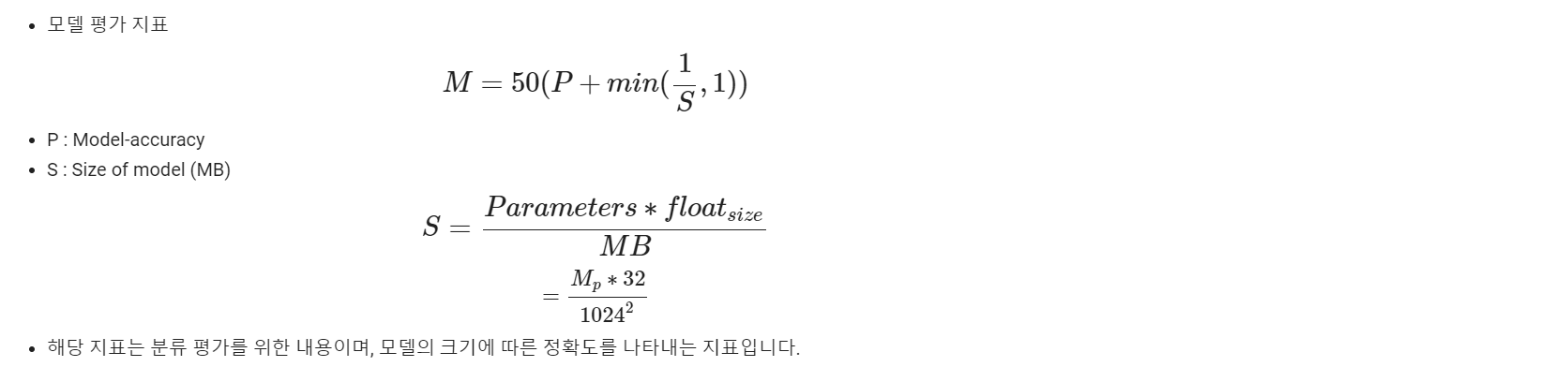
def final_score():
    print("Model params num : " + str(model.count_params()))
    print("Accuracy : " + str(results[1]))

    s = (model.count_params() * 32) / (1024 ** 2)
    score = 50 * (results[1] + min((1/s), 1))

    print("score : " + str(score))
스코어 결과
- 위의 스코어는 분류모델에 적용되는 스코어입니다.
- 모델의 크기 (MB) 와 정확도를 이용해 스코어를 출력합니다.
- 40 이상의 스코어에 도전해보세요!
final_score()추가 과제
- 높은 스코어를 달성하신 분들께선 더 맞추기 어려운 데이터셋으로 도전해보세요.
(train_data, train_labels), (test_data, test_labels) = \
    tf.keras.datasets.cifar100.load_data()
- 데이터 로드 파트에서 위 코드를 고치면 더 세분화된 분류를 진행하는 데이터셋을 사용할 수 있습니다.

AI, Information and Communication, Electronics, Computer Science, Bio, Algorithms