Naver Project(MNIST with DNN)

import tensorflow as tf
from tensorflow.keras import layers

import numpy as np
import matplotlib.pyplot as plt

tf.__version__

#2.15.0
#2.15.0

Dataset 준비

• 학습을 위해 제공되는 MNIST dataset을 준비

# Load training and eval data from tf.keras
(train_data, train_labels), (test_data, test_labels) = \
    tf.keras.datasets.mnist.load_data()

train_data[10].shape

#(28, 28)
#(28, 28)

train_labels[11]

#5
#5

print(train_data.shape, train_labels.shape)
print(test_data.shape, test_labels.shape)

#(60000, 28, 28) (60000,)
#(10000, 28, 28) (10000,)
#(60000, 28, 28) (60000,)
#(10000, 28, 28) (10000,)

set(train_labels[:100])

#{0, 1, 2, 3, 4, 5, 6, 7, 8, 9}
#{0, 1, 2, 3, 4, 5, 6, 7, 8, 9}

# 데이터 전처리 파트 -> 도메인 지식이 들어가게 됩니다.
train_data = train_data / 255.
train_data = train_data.reshape(-1, 28 * 28)
train_data = train_data.astype(np.float32)
train_labels = train_labels.astype(np.int32)

test_data = test_data / 255.
test_data = test_data.reshape(-1, 784)
test_data = test_data.astype(np.float32)
test_labels = test_labels.astype(np.int32)

print(train_data.shape, train_labels.shape)
print(test_data.shape, test_labels.shape)

#(60000, 784) (60000,)
#(10000, 784) (10000,)
#(60000, 784) (60000,)
#(10000, 784) (10000,)

Dataset 구성

• 원활한 학습을 위해서 데이터셋을 구성해주고, Label을 one-hot으로 변환해준다.

def one_hot_label(image, label):
  label = tf.one_hot(label, depth=10)
  return image, label

batch_size = 64
max_epochs = 10

# for train
N = len(train_data)
train_dataset = tf.data.Dataset.from_tensor_slices((train_data, train_labels))
train_dataset = train_dataset.shuffle(buffer_size=10000)
train_dataset = train_dataset.map(one_hot_label)
train_dataset = train_dataset.repeat().batch(batch_size=batch_size)
print(train_dataset)


# for test
test_dataset = tf.data.Dataset.from_tensor_slices((test_data, test_labels))
test_dataset = test_dataset.map(one_hot_label)
test_dataset = test_dataset.batch(batch_size=batch_size)
print(test_dataset)

#<_BatchDataset element_spec=(TensorSpec(shape=(None, 784), dtype=tf.float32, name=None), TensorSpec(shape=(None, 10), dtype=tf.float32, name=None))>
#<_BatchDataset element_spec=(TensorSpec(shape=(None, 784), dtype=tf.float32, name=None), TensorSpec(shape=(None, 10), dtype=tf.float32, name=None))>
#<_BatchDataset element_spec=(TensorSpec(shape=(None, 784), dtype=tf.float32, name=None), TensorSpec(shape=(None, 10), dtype=tf.float32, name=None))>
#<_BatchDataset element_spec=(TensorSpec(shape=(None, 784), dtype=tf.float32, name=None), TensorSpec(shape=(None, 10), dtype=tf.float32, name=None))>

# for train, label in train_dataset.take(3):
#     print(label)
# print("--------")
# for train, label in train_dataset.take(3):
#     print(label)

데이터 확인

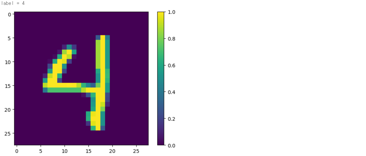
index = 2190
print("label = {}".format(train_labels[index]))
plt.imshow(train_data[index].reshape(28, 28))
plt.colorbar()
#plt.gca().grid(False)
plt.show()

모델 제작

tf.keras.layers.Dense

def __init__(self,
               units,
               activation=None,
               use_bias=True,
               kernel_initializer='glorot_uniform',
               bias_initializer='zeros',
               kernel_regularizer=None,
               bias_regularizer=None,
               activity_regularizer=None,
               kernel_constraint=None,
               bias_constraint=None,
               **kwargs):

# layers.Dense(64,
#              activation='relu',
#              kernel_initializer=tf.keras.initializers.HeNormal(),
#              kernel_regularizer=tf.keras.regularizers.L2(0.0001)
#              )

# Flatten (inputs)
# Dense 128
# Dense 64
# Dense 32
# Dense 16
# (outputs)

# Models Sequential
model = tf.keras.models.Sequential([
    layers.Dense(128, activation='relu'),
    layers.Dense(64, activation='relu'),
    layers.Dense(32, activation='relu'),
    layers.Dense(16, activation='relu'),
    layers.Dense(10)
])

Training

tf.keras.losses.CategoricalCrossentropy()

cce = tf.keras.losses.CategoricalCrossentropy()
loss = cce([[1., 0., 0.], [0., 1., 0.], [0., 0., 1.]],
           [[.9, .05, .05], [.5, .89, .6], [.05, .01, .94]])
print('Loss: ', loss.numpy())  # Loss: 0.3239

model.compile(optimizer=tf.keras.optimizers.Adam(1e-4),
              loss=tf.keras.losses.CategoricalCrossentropy(from_logits=True),
              metrics=['accuracy'])

모델 확인

# without training, just inference a model in eager execution:
predictions = model(train_data[0:1], training=False)
print("Predictions: ", predictions.numpy())

#Predictions:  [[-0.02930707  0.44413155  0.24044743  0.26612186 -0.16049251 -0.03706606
   #0.11634646  0.3885547   0.5697793   0.01176794]]
#Predictions:  [[ 0.01978105  0.03389753 -0.06185833  0.11021287  0.10632764  0.03223215
   #0.0615902  -0.01403253 -0.10297628  0.18898144]]

tf.keras.utils.plot_model(model, show_shapes=True)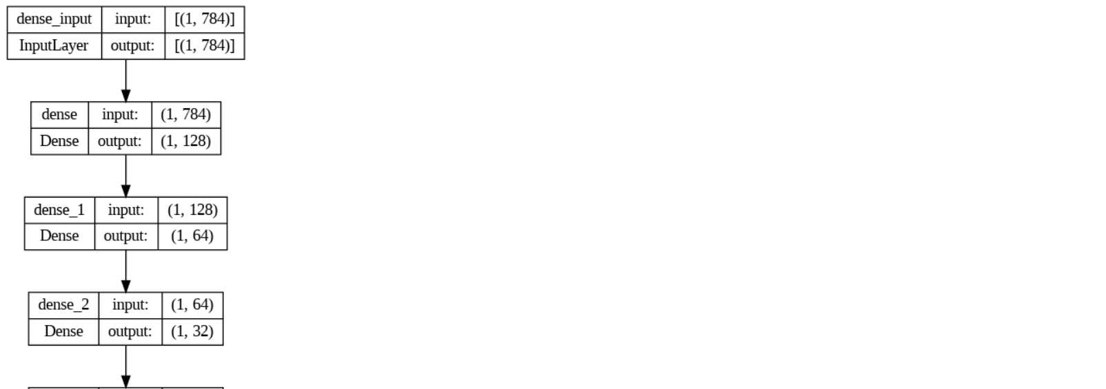

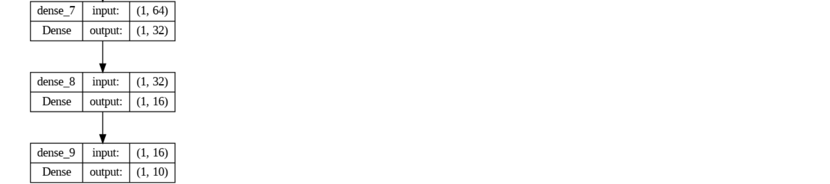
model.summary()

#Model: "sequential_1"
#_________________________________________________________________
# Layer (type)                Output Shape              Param #   
#=================================================================
# dense_5 (Dense)             (None, 128)               100480    
#                                                                 
# dense_6 (Dense)             (None, 64)                8256      
#                                                                 
# dense_7 (Dense)             (None, 32)                2080      
#                                                                 
# dense_8 (Dense)             (None, 16)                528       
#                                                                 
# dense_9 (Dense)             (None, 10)                170       
#                                                                 
#=================================================================
#Total params: 111514 (435.60 KB)
#Trainable params: 111514 (435.60 KB)
#Non-trainable params: 0 (0.00 Byte)
#_________________________________________________________________

학습진행

• model.fit 함수가 최근에 model.fit_generator 함수와 통합
• Dataset을 이용한 학습을 진행

# using `numpy type` data
# history = model.fit(train_data, train_labels,
#                     batch_size=batch_size, epochs=max_epochs,
#                     validation_split=0.05)
# using `tf.data.Dataset` # model.fit_generator
history = model.fit(train_dataset,
                    epochs=max_epochs,
                    steps_per_epoch=len(train_data) // batch_size)

#Epoch 1/10
#937/937 [==============================] - 11s 8ms/step - loss: #0.9375 - accuracy: 0.7416
#Epoch 2/10
#937/937 [==============================] - 5s 5ms/step - loss: 0.3046 #- accuracy: 0.9195
#Epoch 3/10
#937/937 [==============================] - 5s 6ms/step - loss: 0.2245 #- accuracy: 0.9388
#Epoch 4/10
#937/937 [==============================] - 5s 5ms/step - loss: 0.1858 #- accuracy: 0.9472
#Epoch 5/10
#937/937 [==============================] - 4s 5ms/step - loss: 0.1601 #- accuracy: 0.9544
#Epoch 6/10
#3937/937 [==============================] - 6s 6ms/step - loss: #0.1408 - accuracy: 0.9594
#Epoch 7/10
#937/937 [==============================] - 5s 5ms/step - loss: 0.1265 #- accuracy: 0.9632
#Epoch 8/10
#937/937 [==============================] - 5s 5ms/step - loss: 0.1138 #- accuracy: 0.9671
#Epoch 9/10
#937/937 [==============================] - 6s 6ms/step - loss: 0.1031 #- accuracy: 0.9698
#Epoch 10/10
#937/937 [==============================] - 5s 5ms/step - loss: 0.0934 #- accuracy: 0.9730
#Epoch 1/10
#937/937 [==============================] - 6s 5ms/step - loss: 0.9897 #- accuracy: 0.7217
#Epoch 2/10
#937/937 [==============================] - 4s 5ms/step - loss: 0.3255 #- accuracy: 0.9112
#Epoch 3/10
#937/937 [==============================] - 6s 6ms/step - loss: 0.2432 #- accuracy: 0.9323
#Epoch 4/10
#937/937 [==============================] - 4s 5ms/step - loss: 0.2023 #- accuracy: 0.9427
#Epoch 5/10
#937/937 [==============================] - 4s 5ms/step - loss: 0.1748 #- accuracy: 0.9505
#Epoch 6/10
#937/937 [==============================] - 6s 6ms/step - loss: 0.1551 #- accuracy: 0.9556
#Epoch 7/10
#937/937 [==============================] - 4s 5ms/step - loss: 0.1390 #- accuracy: 0.9606
#Epoch 8/10
#937/937 [==============================] - 5s 5ms/step - loss: 0.1263 #- accuracy: 0.9642
#Epoch 9/10
#937/937 [==============================] - 5s 6ms/step - loss: 0.1146 #- accuracy: 0.9672
#Epoch 10/10
#937/937 [==============================] - 4s 5ms/step - loss: 0.1058 #- accuracy: 0.9700

학습결과 확인

history.history.keys()

#dict_keys(['loss', 'accuracy'])
#dict_keys(['loss', 'accuracy'])

acc = history.history['accuracy']

loss = history.history['loss']

epochs_range = range(max_epochs)

plt.figure(figsize=(8, 8))
plt.subplot(1, 2, 1)
plt.plot(epochs_range, acc, label='Training Accuracy')
plt.legend(loc='lower right')
plt.title('Training and Accuracy')

plt.subplot(1, 2, 2)
plt.plot(epochs_range, loss, label='Training Loss')
plt.legend(loc='upper right')
plt.title('Training and Loss')
plt.show()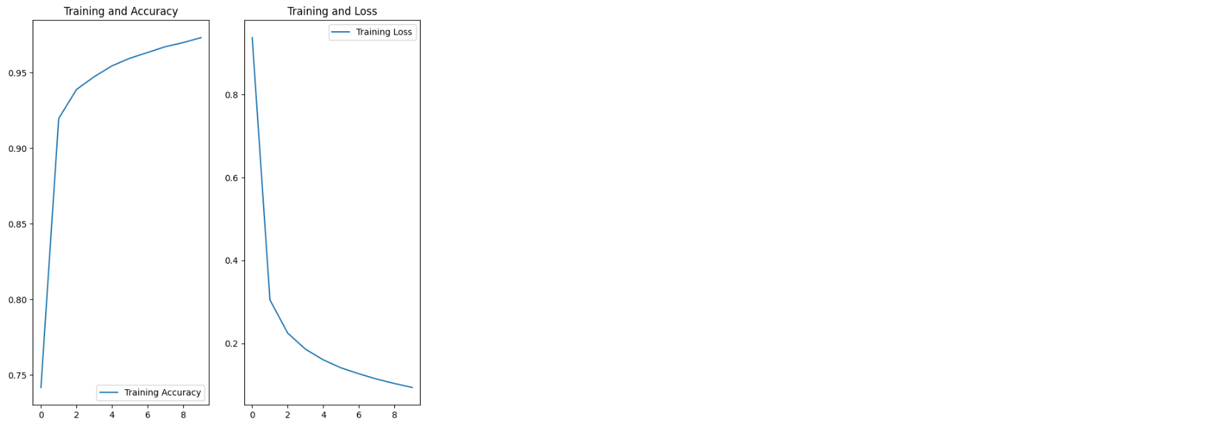

results = model.evaluate(test_dataset, steps=int(len(test_data) / batch_size))

#156/156 [==============================] - 1s 3ms/step - loss: 0.1106 - accuracy: 0.9672
#156/156 [==============================] - 1s 3ms/step - loss: 0.1250 - accuracy: 0.9631

# loss
print("loss value: {:.3f}".format(results[0]))
# accuracy
print("accuracy value: {:.4f}%".format(results[1]*100))

#loss value: 0.111
#accuracy value: 96.7248%
#loss value: 0.125
#accuracy value: 96.3141%

np.random.seed(219)
test_batch_size = 16
batch_index = np.random.choice(len(test_data), size=test_batch_size, replace=False)

batch_xs = test_data[batch_index]
batch_ys = test_labels[batch_index]
y_pred_ = model(batch_xs, training=False)

fig = plt.figure(figsize=(16, 10))
for i, (px, py) in enumerate(zip(batch_xs, y_pred_)):
  p = fig.add_subplot(4, 8, i+1)
  if np.argmax(py) == batch_ys[i]:
    p.set_title("y_pred: {}".format(np.argmax(py)), color='blue')
  else:
    p.set_title("y_pred: {}".format(np.argmax(py)), color='red')
  p.imshow(px.reshape(28, 28))
  p.axis('off')