Naver Project(Multi-variable Linear regression)

Multi-variable Linear Regression

import tensorflow as tf
from tensorflow.keras import layers, Sequential
import numpy as np
import matplotlib.pyplot as plt

tf.__version__

# 2.15.0

Hypothesis

x_data = [
    [1., 0., 3., 0., 5.],
    [0., 2., 0., 4., 0.]
]
y_data  = [1, 2, 3, 4, 5]

W = tf.Variable(tf.random.normal([1, 2], -1.0, 1.0))
b = tf.Variable(tf.random.normal([1], -1.0, 1.0))

print(np.array(x_data).shape, np.array(y_data).shape, W.shape, b.shape)

learning_rate = tf.Variable(0.001)

for i in range(100):
   with tf.GradientTape() as tape:
    # (5, 2) * (2, 1) = (5, 1)
    hypothesis = tf.matmul(W, x_data) + b  # w [1, 2] * x [2, 5] = y [1, 5]
    cost = tf.reduce_mean(tf.square(hypothesis - y_data))

    W_grad, b_grad = tape.gradient(cost, [W, b])
    W.assign_sub(learning_rate * W_grad)
    b.assign_sub(learning_rate * b_grad)

    if i % 10 == 0:
        print("step: {:3} \t cost: {:5.4f} \t w[0][0]: {:5.4f} \t w[0][1]: {:5.4f} \t b: {:5.4f}".format(
            i, cost.numpy(), W.numpy()[0][0], W.numpy()[0][1], b.numpy()[0]))

#(2, 5) (5,) (1, 2) (1,)
#step:   0 	 cost: 43.4899 	 w[0][0]: -1.0720 	 w[0][1]: -0.5564 	 b: #-0.2215
#step:  10 	 cost: 32.7634 	 w[0][0]: -0.7938 	 w[0][1]: -0.4323 	 b: #-0.1122
#step:  20 	 cost: 24.7433 	 w[0][0]: -0.5556 	 w[0][1]: -0.3202 	 b: #-0.0171
#step:  30 	 cost: 18.7372 	 w[0][0]: -0.3518 	 w[0][1]: -0.2188 	 b: #0.0657
#step:  40 	 cost: 14.2316 	 w[0][0]: -0.1774 	 w[0][1]: -0.1270 	 b: #0.1377
#step:  50 	 cost: 10.8451 	 w[0][0]: -0.0283 	 w[0][1]: -0.0439 	 b: #0.2004
#step:  60 	 cost: 8.2943 	 w[0][0]: 0.0993 	 w[0][1]: 0.0314 	 b: #0.2550
#step:  70 	 cost: 6.3686 	 w[0][0]: 0.2084 	 w[0][1]: 0.0997 	 b: #0.3026
#step:  80 	 cost: 4.9111 	 w[0][0]: 0.3016 	 w[0][1]: 0.1618 	 b: 
#0.3440
#step:  90 	 cost: 3.8050 	 w[0][0]: 0.3812 	 w[0][1]: 0.2181 	 b: #0.3801

Test Score

Hypothesis using matrix

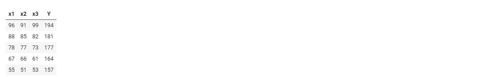
data = np.array([
    # X1,   X2,    X3,   Y
    [ 96.,  91.,  99., 194. ],
    [ 88.,  85.,  82., 181. ],
    [ 78.,  77.,  73., 177. ],
    [ 67.,  66., 61., 164. ],
    [ 55.,  51.,  53., 157. ]
], dtype=np.float32)

# slice data
X = data[:, :-1]
print(X.shape)
y = data[:, [-1]]
print(y.shape)

# Model
W = tf.Variable(tf.random.normal([3, 1]))
b = tf.Variable(tf.random.normal([1]))

learning_rate = 0.00001

def predict(X):
    return tf.matmul(X, W) + b

print("epoch | cost")

n_epochs = 1000
for i in range(n_epochs):
    # tf.GradientTape() to record the gradient of the cost function
    with tf.GradientTape() as tape:
        cost = tf.reduce_mean((tf.square(predict(X) - y)))

    # Loss함수의 gradient를 계산한다.
    W_grad, b_grad = tape.gradient(cost, [W, b])

    # 파라미터 업데이트 (W and b) -> Optimizer!
    W.assign_sub(learning_rate * W_grad)
    b.assign_sub(learning_rate * b_grad)

    if i % 100 == 0:
        print("{:5} | {:10.4f}".format(i, cost.numpy()))

#(5, 3)
#(5, 1)
#epoch | cost
#    0 | 44150.8203
#  100 |   431.2387
#  200 |   428.8976
#  300 |   426.6577
#  400 |   424.5135
#  500 |   422.4610
#  600 |   420.4948
#  700 |   418.6113
#  800 |   416.8062
#  900 |   415.0754

데이터를 기반으로예측해보자

def predict(X):
    return tf.matmul(X, W) + b # 위쪽에 선언되어 있다.

predict(X).numpy() # prediction, 예측값

#array([[212.09036],
#       [195.96054],
#       [174.76112],
#       [150.04295],
#       [120.72071]], dtype=float32)

W

#<tf.Variable 'Variable:0' shape=(3, 1) dtype=float32, numpy=
#array([[ 1.6190001 ],
#       [ 0.6897571 ],
#       [-0.05651399]], dtype=float32)>

# 새로운 데이터에 대한 예측

predict([[ 89.,  95.,  92.],[ 84.,  92.,  85.]]).numpy()

#array([[203.91197],
#       [194.1433 ]], dtype=float32)

with Tensorflow

data = np.array([
    # X1,   X2,    X3,   y
    [ 96.,  91.,  99., 194. ],
    [ 88.,  85.,  82., 181. ],
    [ 78.,  77.,  73., 177. ],
    [ 67.,  66., 61., 164. ],
    [ 55.,  51.,  53., 157. ]
], dtype=np.float32)

# slice data
X = data[:, :-1]
y = data[:, [-1]] # Raw data

# tf.data generate data from raw data
dataset = tf.data.Dataset.from_tensor_slices((X, y))
dataset = dataset.batch(batch_size=1)

model = Sequential([
    layers.Dense(1, activation='linear')
])

model.compile(optimizer='adam', # W assign_sub
              loss='mse', # mse, mae
              metrics=['mse'])

model.fit(dataset, epochs=1000) # tf.GradientTape 교체가능!

tf.keras.utils.plot_model(model, show_shapes=True)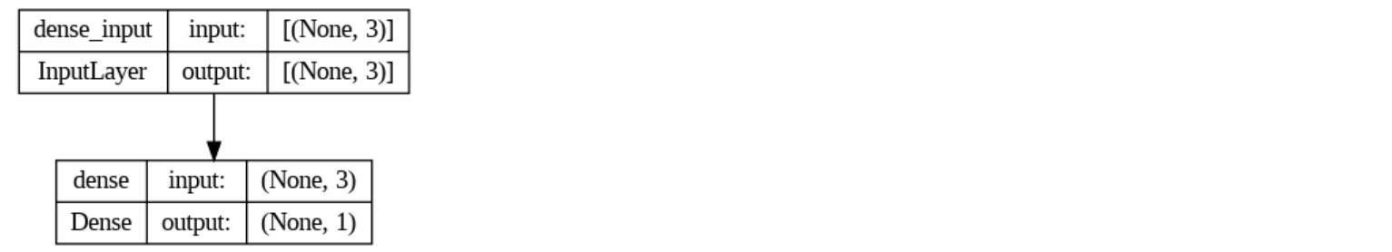

test_loss, test_mae = model.evaluate(X, y, verbose=0)
print('Test MSE:', test_mae)

# Test MSE: 520.80517578125

for x, y in dataset:
    print(x)
    print(y)
    print(model(x))
    break

#tf.Tensor([[96. 91. 99.]], shape=(1, 3), dtype=float32)
#tf.Tensor([[194.]], shape=(1, 1), dtype=float32)
#tf.Tensor([[223.35674]], shape=(1, 1), dtype=float32)