1. 데이터 분석 프로세스
ML
┌────┼────┐
지도 비지도 강화
↓
회귀
분류
목표
- 예측 모델링에 필요한 전체 프로세스 이해
예측 모델링 프로세스
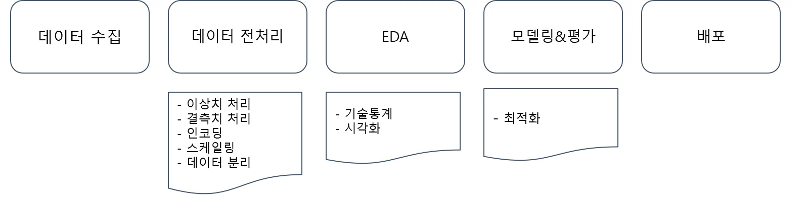
- 머신러닝의 이해와 라이브러리 활용 기초 강의에서 예측 모델링 프로세스 중 '모델링과 평가' 부분을 배웠음
- 핵심 부분을 이해했으니 이제 전체 내용에 대해 확인해보자! →
데이터 전처리,
EDA 학습
데이터 수집
데이터 수집에 따른 프로세스
☞ SNOWFLAKE - “MODERN” DATA ARCHITECTURES
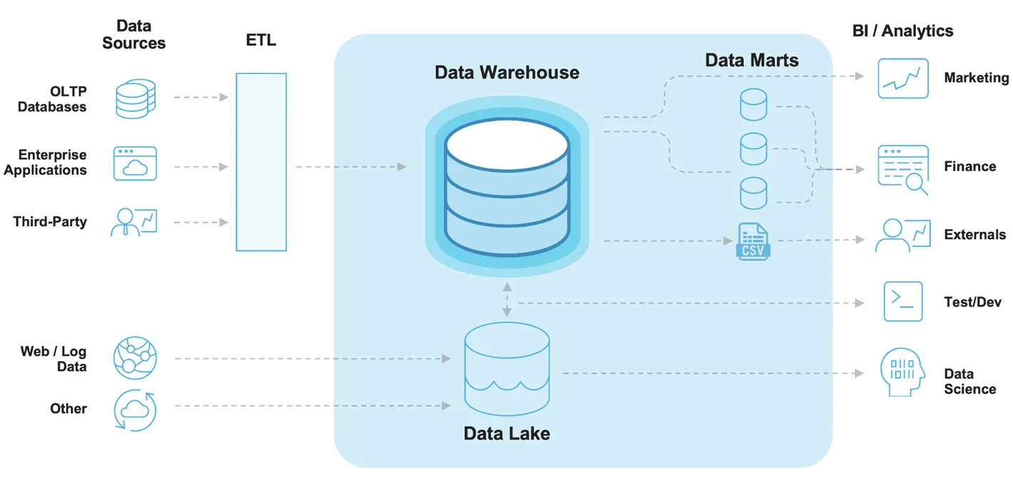
🡆 Snowflake라는 유명한 데이터 소프트웨어 회사의 데이터 스키마
ETL 과정: 데이터 추출(Extract), 변환(Transform), 로드(Load) 과정 → 데이터 엔지니어의 업무임
🡆 데이터 분석가는 데이터가 "흐르는" 기업으로 가야 함!
그렇지 않으면 적재부터 시작해야 해서 너무 힘들다고 한다…
🡆 연습할 때는 이미 수집되어 정제가 왼료된 데이터를 사용하기 때문에 지나치는 경우가 많은데 실제로는 이 부분이 가장 궁요함!
데이터 수집 단계는 예제 데이터 혹은 회사에 있는 데이터로 진행되기 때문에, 지나치는 경우가 많지만 실제로 데이터를 수집하려면 개발을 통해 데이터를 적재하고 수집하는 데이터 엔지니어링 역량이 필요합니다.
보통 이 부분은 개발자가 직접 설계하고 저장하게 되며, 데이터 분석가는 이미 존재하는 데이터를 SQL 혹은 Python으로 추출하고 리포팅 혹은 머신러닝을 통한 예측 부분을 담당한다고 할 수 있습니다.
- Data Source
- OLTP(OnLine Transaction Processing) Database
- 온라인 뱅킹,쇼핑, 주문 입력 등 동시에 발생하는 다수의 트랜잭션(데이터베이스 작업의 단위) 처리 유형
- Enterprise Applications
- 회사 내 데이터 (예: 고객 관계 데이터, 제품 마케팅 세일즈)
- Third-Party
- Google Analytics와 같은 외부소스에서 수집되는 데이터
- Web/Log
- 사용자의 로그데이터
- OLTP(OnLine Transaction Processing) Database
- Data Lake
- 원시 형태의 다양한 유형의 데이터를 저장
- Data Warehouse
- 보다 구조화된 형태로 정제된 데이터를 저장
- 전사적으로 데이터를 다 모아놓는 공간
- Data Marts: 조직을 위해 가공한 목적성이 있는 데이터
- Data Marts
- 회사의 금융, 마케팅, 영업 부서와 같이 특정 조직의 목적을 위해 가공된 데이터
- '데이터 마트를 만다'는 표현을 쓴다고 함
- BI/Analytics
- BI(business Intelligence)
- 의사결정에 사용될 데이터를 수집하고 분석하는 프로세스
- BI(business Intelligence)
실제 데이터 수집
- 회사 내 데이터가 존재한다면
- SQL 혹은 Python 을 통해 데이터 마트를 생성
→ 정형 데이터 추출 속도는 SQL이 압도적으로 좋다고 함!
- SQL 혹은 Python 을 통해 데이터 마트를 생성
- 회사 내 Data가 없다면 → 데이터 수집 필요
- CSV, EXCEL 파일 다운로드
- API를 이용한 데이터 수집
→ API(Application Interface): 두 소프트웨어 간 규격화된 형태로 의사소통을 하는 것(API 단위로 의사소통 & 데이터 수집) - Data Crawling
☞ 공공데이터포털 - API 사용 목록(data.go.kr)

EDA(탐색적 데이터 분석)
- 탐색적 데이터 분석(Exploratory Data Analysis, EDA)
- 데이터의 시각화, 기술통계 등의 방법을 통해 데이터를 이해하고 탐구하는 과정
- 데이터에 대한 정보를 얻을 수도 있고, 적절한 모델링에 대한 정보도 얻을 수 있음
- 예측 모델링이 아니더라도 데이터 분석에서는 반드시 필요한 과정
이전 데이터 분석과 시각화 강의에서 들었다고 가정하고 시각화는 seaborn라이브러리를 활용 간단하게 알아보도록 할게요.
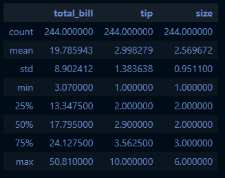
기술통계를 통한 EDA 예시
tips.describe():describe()메서드 활용include='all'옵션을 통해 범주형 데이터도 확인 가능
import sklearn
import numpy as np
import pandas as pd
import matplotlib.pyplot as plt
import seaborn as sns
from sklearn.metrics import mean_squared_error, r2_score

# seaborn 시각화 라이브러리는 기본적으로 데이터셋을 제공: seaborn.load_dataset
tips_df = sns.load_dataset('tips')
tips_df.describe(include='all')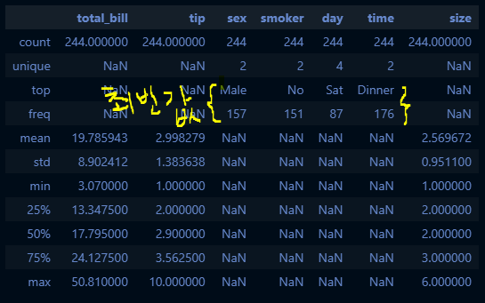
cf. tips_df.describe()
시각화를 이용한 EDA 예시
- tips 데이터
🡆 시각화 방법은 아래 세 가지를 각각 x, y축에 넣는 것!
A. 범주형
B. 연속형
C. 관측치
- X축, Y축에 필요한 정보를 넣어서 시각화
- 범주형 데이터
- 연속형 자료형
- 관측치 → Y축에 넣음
- countplot: 범주형 자료의 '빈도수' 시각화
- 방법
- 범주형의 데이터의 각 카테고리별 빈도수를 나타낼 때
(예) 상점에서 판매되는 제품의 카테고리별 판매수 파악
- 범주형의 데이터의 각 카테고리별 빈도수를 나타낼 때
- x축
- 범주형 자료
- y축
- 자료의 빈도수
- 방법
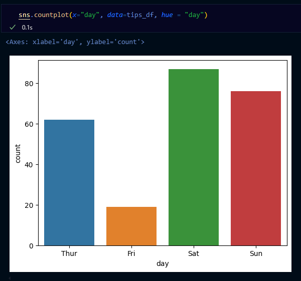
→ countplot: x축 범주형, y축 관측치
- barplot: 범주형 자료의 시각화
- 방법
- 범주형 데이터의 각 카테고리에 따른 수치 데이터의 평균을 비교
(예) 다양한 연령대별 평균소득을 비교
- 범주형 데이터의 각 카테고리에 따른 수치 데이터의 평균을 비교
- x축
- 범주형 자료
- y축
- 연속형 자료
- 방법
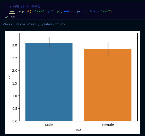
→ barplot: x축이 범주형, y축이 연속형 값
→ 기본값은 평균인데 estimator='sum'으로 넣으면 평균이 아니라 전체합을 볼 수 있음
- boxplot: 수치형 & 범주형 자료의 시각화
- 방법
- 데이터의 분포, 중앙값, 사분위 수, 이상치 등을 한눈에 표현하고 싶을 때
(예) 여러 그룹간 시험 점수 분포를 비교
- 데이터의 분포, 중앙값, 사분위 수, 이상치 등을 한눈에 표현하고 싶을 때
- x축
- 수치형 or 범주형
- y축
- 수치형 자료
- 방법
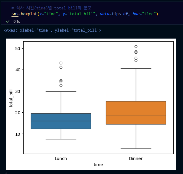
→ 동그라미는 outlier
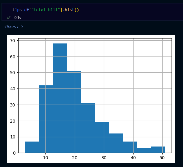
- histogram: 수치형 자료 빈도 시각화
- 방법
- 연속형 분포를 나타내고 싶을 때, 데이터가 몰려있는 구간을 파악하기 쉬움
(예) 고객들의 연령 분포를 파악
- 연속형 분포를 나타내고 싶을 때, 데이터가 몰려있는 구간을 파악하기 쉬움
- x축
- 수치형 자료
- y축
- 자료의 빈도수
- 방법
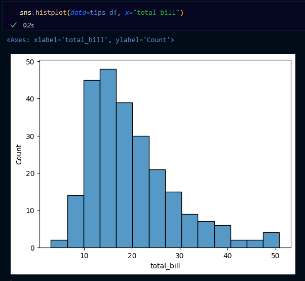
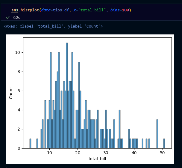
→ bins= 이용해 구간 설정할 수 있음
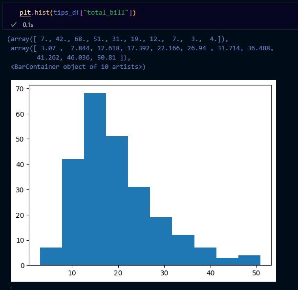
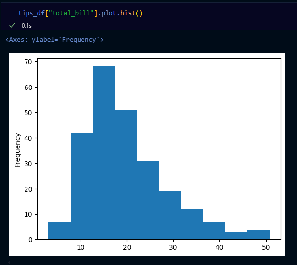
다음의 코드도 동일한 그래프를 그려요!
plt.hist(tips_df["total_bill"])
tips_df["total_bill"].hist()
tips_df["total_bill"].plot.hist()
- scatterplot: 수치형끼리 자료의 시각화
- 방법
- 두 연속형 변수간의 관계를 시각적으로 파악하고 싶을 때
(예) 키와 몸무게 간의 관계
- 두 연속형 변수간의 관계를 시각적으로 파악하고 싶을 때
- x축
- 수치형 자료
- y축
- 수치형 자료
- 방법
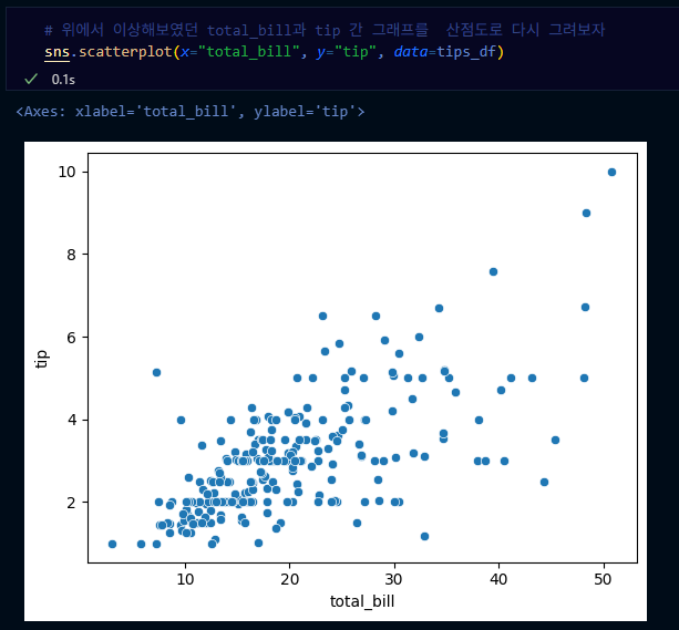
→ scatterplot: x축 수치형 변수, y축 수치형 변수
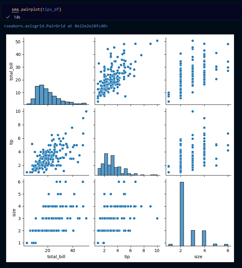
- pairplot: 전체 변수에 대한 시각화
- 방법
- 한 번에 여러 개의 변수를 동시에 시각화 하고 싶을 때
- x축
- 범주형 or 수치형 자료
- y축
- 범주형 or 수치형 자료
- 대각선
- 히스토그램(분포)
- 방법
데이터 전처리
데이터 전처리는 전체 분석 프로세스에서 90%를 차지 할 정도로 노동, 시간 집약적인 단계예요.
이번 장에서 해당 부분을 직접적으로 알아 볼게요.
이상치(Outlier)
- 보통
관측된 데이터 범위에서 많이 벗어난 아주 작은 값 혹은 큰 값을 말함 - 크게 2가지 기준이 있음
- ESD(Extreme
Studentized Deviation) 이용한 이상치 발견
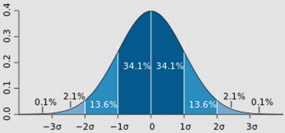
- 데이터가 정규분포를 따른다고 가정할 때, 평균에서 표준편차의 3배 이상 떨어진 값
🡆 Studentized라는 단어를 보면 분포→정규분포 연관성 생각하면 좋음
- 모든 데이터가 정규 분포를 따르지 않을 수 있기 때문에 다음 상황에서는 제한됨
a. 데이터가 크게 비대칭일 때( → Log변환 등을 노려볼 수 있음)
b. 샘플 크기가 작을 경우
- IQR(Inter Quantile Range)를 이용한 이상치 발견
- ESD와 동일하게 데이터가 비대칭적이거나 샘플사이즈가 작은 경우 제한됨
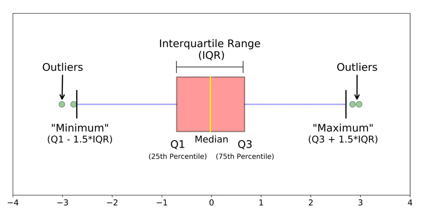
- Box plot
: 데이터의 사분위 수를 포함하여 분포를 보여주는 시각화 그래프.
상자-수염 그림이라고도 함.
※ 사분위 수
: 테이블을 순서에 따라 4등분 한 것
- ESD와 동일하게 데이터가 비대칭적이거나 샘플사이즈가 작은 경우 제한됨
- ESD(Extreme
- 이상치 발견 방법
- ESD를 이용한 처리
import numpy as np mean = np.mean(data) std = np.std(data) upper_limit = mean + 3*std lower_limit = mean - 3*std - IQR을 이용한 처리(box plot)
- pd.Series 이용
Q1 = df['column'].quantile(0.25) Q3 = df['column'].qunatile(0.75) IQR = Q3 - Q1 uppper_limit = Q3 + 1.5*IQR lower_limit = Q1 - 1.5*IQR - 조건필더링을 통한 삭제
(a.k.a. Boolean Indexing)
df[ df['column'] > limit_value]
- ESD를 이용한 처리
이상치는 사실 주관적인 값입니다. 그 데이터를 삭제 할지 말지는 분석가가 결정할 몫입니다. 다만, 이상치는 도메인과 비즈니스 맥락에 따라 그 기준이 달라지며, 데이터 삭제 시 품질은 좋아질 수 있지만 정보 손실을 동반하기 때문에 이상치 처리에 주의해야 합니다. 단지, 통계적 기준에 따라서 결정할 수도 있다는 점 알아두세요.
또한, 이상 탐지(Anomaly Detection)이라는 이름으로 데이터에서 패턴을 다르게 보이는 개체 또는 자료를 찾는 방법으로도 발전 할 수 있습니다.(사기탐지, 사이버 보안 등)
이상치 처리 실습
# ESD 이상치 처리
mean = np.mean(tips_df["total_bill"])
std = np.std(tips_df["total_bill"])
upper_limit = mean + 3*std
lower_limit = mean - 3*std

print(upper_limit, lower_limit)
→ 실행 결과:
46.43839435626422 -6.866509110362578
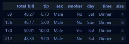
# Boolean Indexing
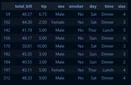
cond = (tips_df['total_bill'] > 46.4)
tips_df[cond]→ 실행 결과:
# IQR을 이용한 이상치 확인(boxplot)
sns.boxplot(tips_df["total_bill"])
→ 실행 결과:
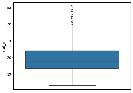
q1 = tips_df["total_bill"].quantile(0.25)
q3 = tips_df["total_bill"].quantile(0.75)
iqr = q3 - q1
upper_limit_iqr = q3 + 1.5*iqr
lower_limit_iqr = q1 - 1.5*iqr

print(f"q1: {q1}, q3:{q3}, iqr:{iqr}")
print(f"upper limit: {upper_limit_iqr}, lower limit: {lower_limit_iqr}")
→ 실행 결과:
q1: 13.3475, q3:24.127499999999998, iqr:10.779999999999998
upper limit: 40.29749999999999, lower limit: -2.8224999999999945
cond_iqr = (tips_df["total_bill"]>upper_limit_iqr)
tips_df[cond_iqr]
→ 실행 결과:
결측치(Missing Value)
이상치가 분포에 크게 어긋나는 특이한 데이터라면, 결측치(Missing Value)는 존재하지 않는 데이터예요.
- 결측치 처리 방법
- 수치형 데이터
- 평균값 대치: 대표적인 대치 방법
- 중앙값 대치: 데이터에 이상치가 많아 평균값이 대표성이 없다면 중앙값을 이용
→ skewed data
(예) 이상치는 평균값을 흔들리게 함 → 평균은 만능이 아니다!

- 범주형 데이터
- 최빈값 대치
- 수치형 데이터
- 사용 함수
- 간단한 삭제 & 대치
df.dropna(axis=0): 결측치가 포함된 모든 행 제거df.dropna(axis=1): 결측치가 포함된 모든 열 제거- Boolean Indexing
df.fillna(value): 특정 값으로 대치(평균, 중앙, 최빈값)
- 알고리즘 이용
sklearn.impute.SimpleImputer: 평균, 중앙, 최빈값으로 대치
SimpleImputer.statistics_: 대치한 값 확인 가능sklearn.impute.IterativeImputer: 다변량대치(회귀 대치)
→ 다른 모든 특성에서 각 특성을 추정(회귀분석에 의한 예측치로 결측치를 대치)sklearn.impute.KNNImputer: KNN 알고리즘을 이용한 대치
→ KNN == K-Nearest Neighbors(k-최근접 이웃)
- 간단한 삭제 & 대치
위와 같이 간단하게 결측치를 대치할 수도 있지만, 알고리즘을 이용해 대치할 수도 있습니다. 이는 Imputation이라는 방법론으로 통계학에서도 많이 발전되었고, 석사 전공으로도 따로 있답니다.
예를 들면, 대표적인 알고리즘인 K-Nearest Neighbors(k-최근접 이웃)이라는 방법이 있습니다. 이 부분은 모델 심화에서 다루도록 할게요!
실습
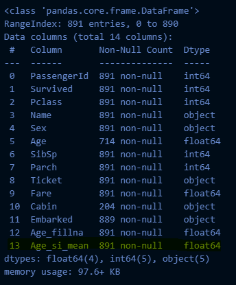
# 결측치: tips에는 결측치가 없어서 titanic 사용
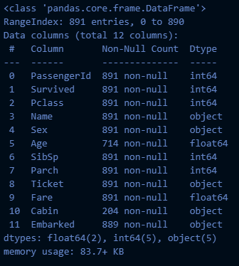
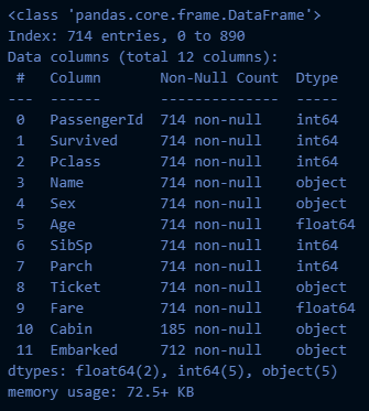
titanic_df = pd.read_csv("train.csv")
titanic_df.info()→ 실행 결과:
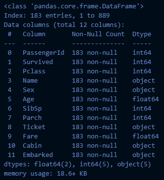
# 결측치 처리: 삭제
titanic_df.dropna(axis=0).info()
→ 실행 결과:
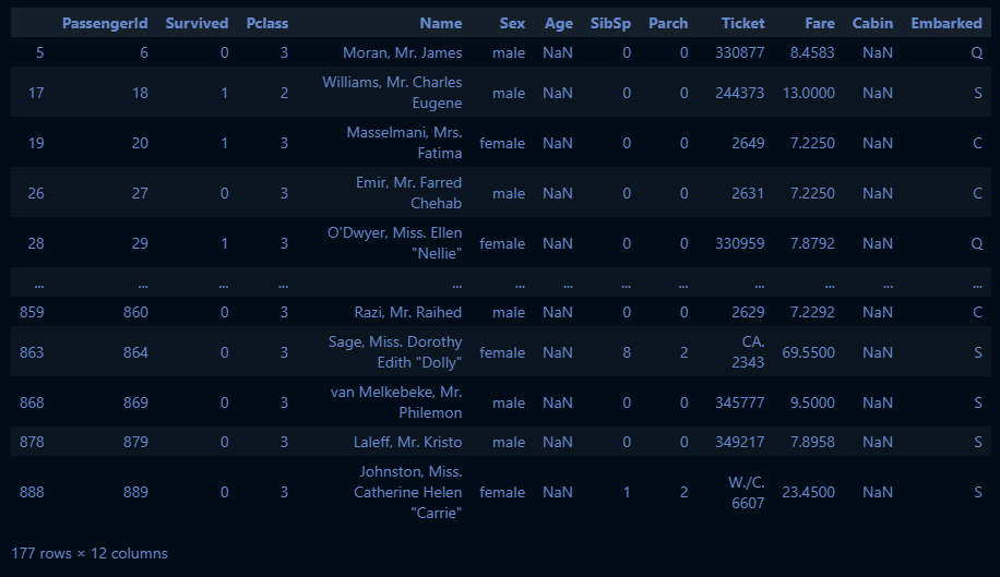
cond_age_na = (titanic_df["Age"].isna())
titanic_df[cond_age_na]
→ 실행 결과:
cond_age_notna = (titanic_df["Age"].notna())
titanic_df[cond_age_notna].info()
→ 실행 결과:
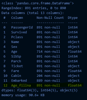
# fillna 이용한 대치
age_mean = titanic_df["Age"].mean().round(2)
titanic_df["Age_fillna"] = titanic_df["Age"].fillna(age_mean)
titanic_df.info()
→ 실행 결과:
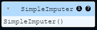
# SimpleImputer를 이용한 대치

from sklearn.impute import SimpleImputer
si = SimpleImputer()
si.fit(titanic_df[["Age"]])
→ 실행 결과:
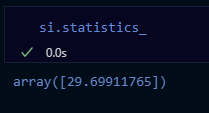
titanic_df["Age_si_mean"] = si.transform(titanic_df[["Age"]])
titanic_df.info()
→ 실행 결과:
범주형 데이터 전처리: 인코딩(Encoding)
인코딩의 사전적 뜻은 어떤 정보를 정해진 규칙에 따라 변환하는 것을 뜻합니다.
우리가 만든 머신러닝 모델은 숫자를 기반으로 학습하기
때문에 반드시 인코딩 과정이 필요합니다.
인코딩(Encoding) ↔ 디코딩(Decoding)
- 레이블 인코딩(Label Encoding)
- 정의: 문자열 범주형 값을 고유한 숫자로 할당
- 1등급 → 0
- 2등급 → 1
- 3등급 → 2
- 특징
- 장점
- 모델이 처리하기 쉬운 수치형으로 데이터 변환
- 단점
- 실제로는 그렇지 않은데, 순서 간 크기에 의미가 부여되어 모델이 잘못 해석할 수 있음
- 장점
- 사용 함수
sklearn.preprocessing.LabelEncoder- 메서드
fit: 데이터 학습transform: 정수형 데이터로 변환fit_transform: fit과 transform을 연결하여 한번에 실행inverse_transform: 인코딩된 데이터를 원래 문자열로 변환
- 속성
classes_: 인코더가 학습한 클래스(범주)
- 원핫 인코딩(One-Hot Encoding)
- 정의: 각 범주를 이진 형식으로 변환하는 기법
- 빨강 → [1,0,0]
- 파랑 → [0,1,0]
- 초록 → [0,0,1]
- 특징
- 장점
- 각 범주가 독립적으로 표현되어, 순서가 중요도를 잘못 학습하는 것을 방지
- 명목형 데이터에 권장
- 단점
- 범주 개수가 많을 경우 차원이 크게 증가(차원의 저주; curse of demensionality)
- 모델의 복잡도를 증가
- 과적합 유발
- 장점
- 사용 함수
pd.get_dummiessklearn.preprocessing.OneHotEncoder- 메서드(LabelEncoder와 동일)
categories_: 인코더가 학습한 클래스(범주)get_feature_names_out(): 학습한 클래스 이름(리스트)
# CSR 데이터 데이터프레임으로 만들기
csr_df = pd.DataFrame(csr_data.toarray(), columns = oe.get_feature_names_out())

# 기존 데이터프레임에 붙이기(옆으로)
pd.DataFrame([titaninc_df,csr_df], axis = 1)
실습
# 성별(Sex)은 LabelEncoder
# 항구(Embarked)는 OneHotEncoder

from sklearn.preprocessing import LabelEncoder, OneHotEncoder

le = LabelEncoder()
oe = OneHotEncoder()

le.fit(titanic_df[["Sex"]])
→ 실행 결과:
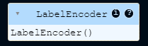
le.classes_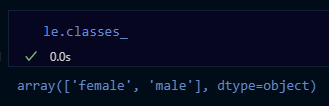
titanic_df["Sex_le"] = le.transform(titanic_df[["Sex"]])
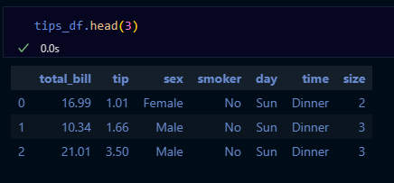
titanic_df.head(3)→ 실행 결과:

oe.fit(titanic_df[["Embarked"]])
oe.categories_
oe.transform(titanic_df[["Embarked"]])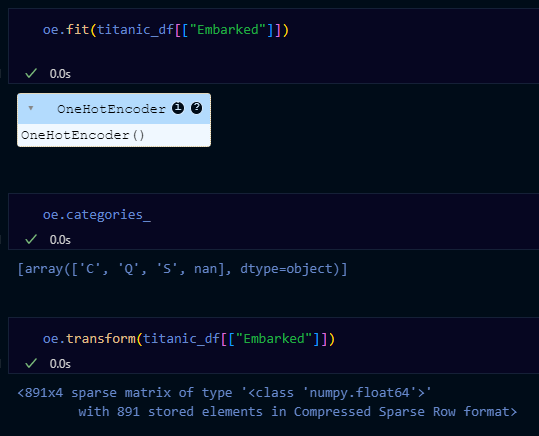
※ sparse → 891x4 행렬의 대부분이 비어 있어서 '데이터가 희박하다'는 뜻임
🡆 sparse metrix의 타입은 보통 CSR(Compressed Sparse Row, 압축된 희소 행)이라 불림
| c | q | s | nan | |
|---|---|---|---|---|
| 0 | [1, 0, 0, 0] | |||
| 1 | [0, 1, 0, 0] | |||
| 2 | [0, 0, 0, 1] | |||
| ¨ | … | |||
| 890 |
embarked_csr = oe.transform(titanic_df[["Embarked"]])
pd.DataFrame(embarked_csr.toarray(), columns=oe.get_feature_names_out())
→ 실행 결과:
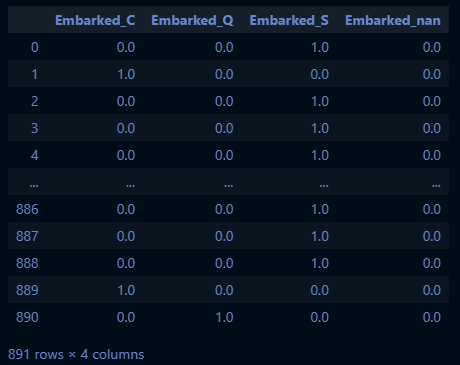
embarked_csr_df = pd.DataFrame(embarked_csr.toarray(), columns=oe.get_feature_names_out())
pd.concat([titanic_df, embarked_csr_df], axis=1).head(3)
수치형 데이터 전처리: 스케일링(Scaling)
인코딩이 범주형 자료에 대한 전처리라고 한다면, 스케일링은 수치형 자료에 대한 전처리입니다.
머신러닝의 학습에 사용되는 데이터들은 서로 단위 값이 다르기 때문에 이를 보정한다고 생각해주세요.
- 표준화(Standardization)
: 각 데이터에 평균을 빼고 표준편차를 나누어 평균을 0 표준편차를 1로 조정하는 방법
- 수식
- 함수
:sklearn.preprocessing.StandardScaler- 메서드
fit: 데이터학습(평균과 표준편차를 계산)transform: 데이터 스케일링 진행
- 속성
mean_: 데이터의 평균 값scale_,var_: 데이터의 표준 편차, 분산 값n_features_in_: fit 할 때 들어간 변수 개수feature_names_in_: fit 할 때 들어간 변수 이름n_samples_seen_: fit 할 때 들어간 데이터의 개수
- 메서드
- 특징
- 장점
- 이상치가 있거나 분포가 치우쳐져 있을 때 유용
- 모든 특성의 스케일을 동일하게 맞춤. 많은 알고리즘에서 좋은 성능
- 단점
- 데이터의 최솟값, 최댓값이 정해지지 않음
- 장점
- 정규화(Normalization)
: 데이터를 0과 1사이 값으로 조정(최솟값 0, 최댓값 1)
- 수식
- 함수
:sklearn.preprocessing.MinMaxScaler- 매서드 → 표준화와 같음
- 속성
data_min_: 원 데이터의 최솟값data_max_: 원 데이터의 최댓값data_range_: 원 데이터의 최대-최소 범위
- 특징
- 장점
- 모든 특성의 스케일을 동일하게 맞춤
- 최대-최소 범위가 명확
- 단점
- 이상치에 영향을 많이 받을 수 있음(반대로 말하면 이상치가 없을 때 유용)
- 장점
- 로버스트 스케일링(Robust Scaling)
: 중앙값과 IQR을 사용하여 스케일링
- 수식
- 함수
:sklearn.preprocessing.RobustScaler- 속성
center_: 훈련 데이터의 중앙값
- 속성
- 특징
- 장점
- 이상치의 영향에 덜 민감
- 단점
- 표준화와 정규화에 비해 덜 사용됨
- 장점
실습
# 수치형 데이터 전처리: 스케일링
# StandardScaler, MinMaxScaler

sns.pairplot(titanic_df)
→ 실행 결과:
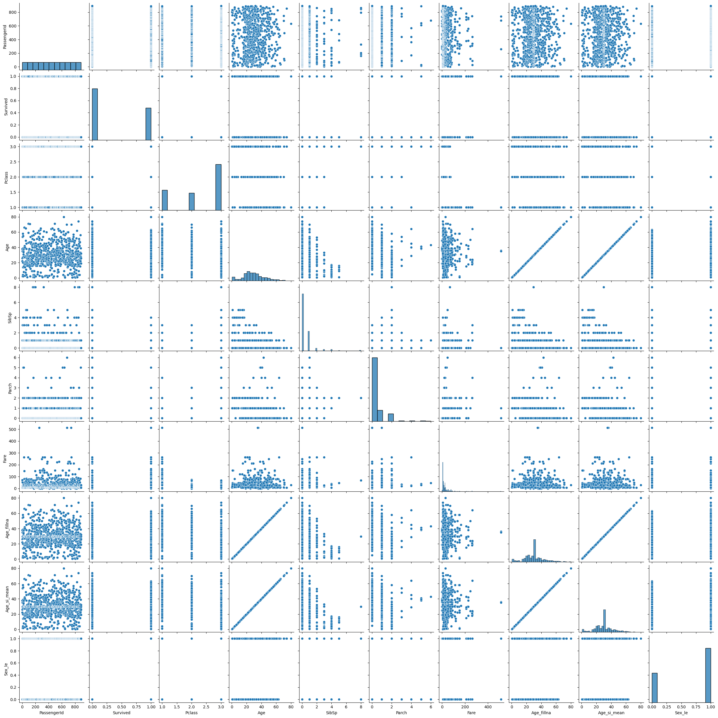
🡆 pairplot의 단점: 값이 너무 많으면 보기가 힘듦
→ 이산형 데이터 말고 연속형 데이터만 가져와서 다시 보기!
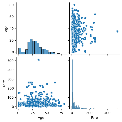
titanic_df.info()→ 연속형 데이터 확인: Age, Fare
sns.pairplot(titanic_df[["Age", "Fare"]])→ 실행 결과:
# 기술통계 확인
titanic_df[["Age", "Fare"]].describe()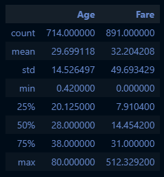
# Age는 MinMaxScaler, Fare는 StandardScaler
from sklearn.preprocessing import MinMaxScaler, StandardScaler
mm_sc = MinMaxScaler()
std_sc = StandardScaler()

titanic_df["Age_mm_sc"] = mm_sc.fit_transform(titanic_df[["Age_fillna"]])
titanic_df.head(3)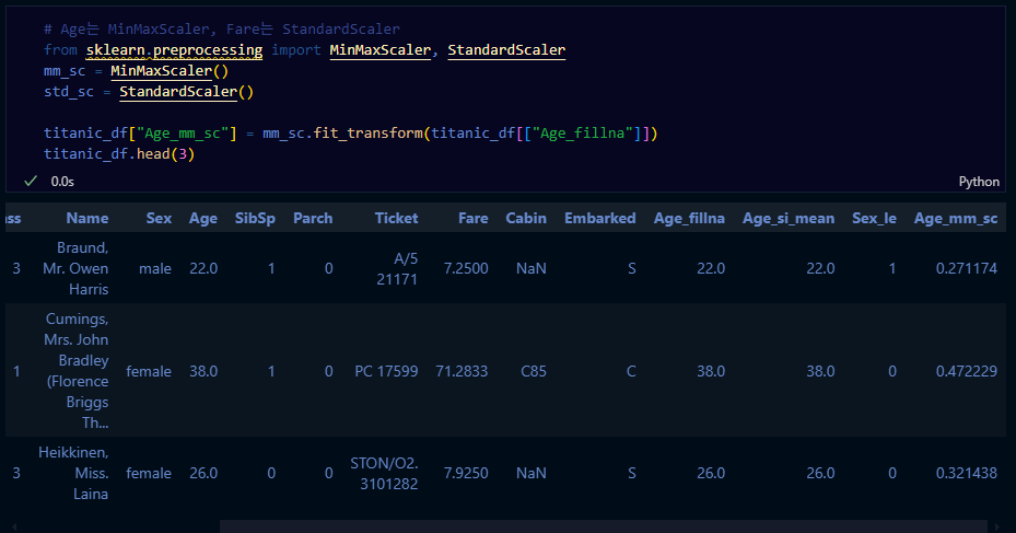
titanic_df["Fare_std_sc"] = std_sc.fit_transform(titanic_df[["Fare"]])
titanic_df.head(3)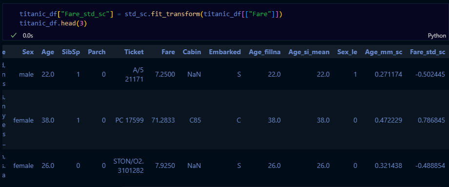
sns.histplot(titanic_df["Age_mm_sc"])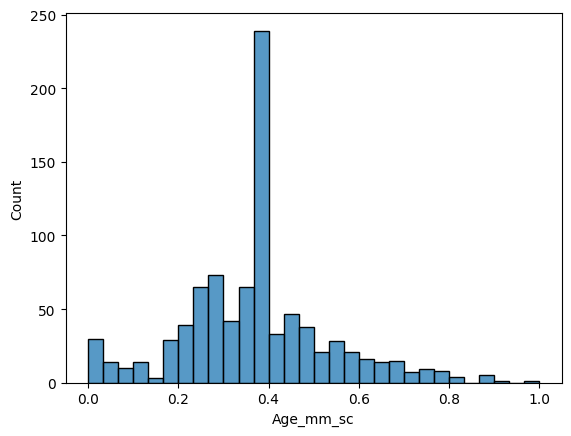
sns.histplot(titanic_df["Age_mm_sc"], bins=100)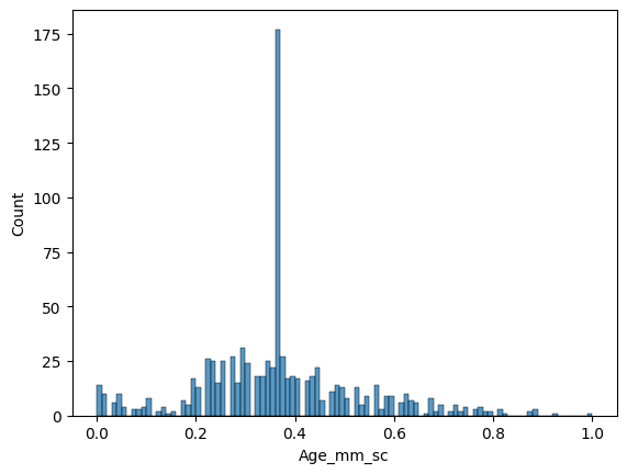
sns.histplot(titanic_df["Fare_std_sc"])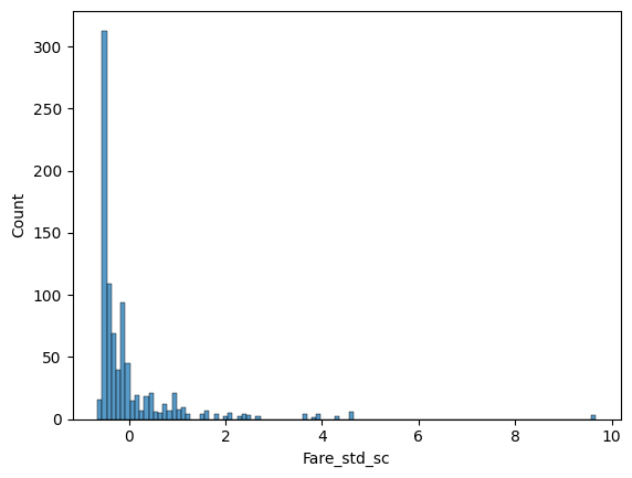
실습한 내용 정리
- 탐색적 데이터 분석과 데이터 전처리
- 탐색적 데이터 분석
- tips 데이터
- 데이터 전처리
- 이상치 처리, 결측치 처리(titaninc 데이터)
- 범주형 변수: 인코딩
- 연속형 변수: 스케일링
- 탐색적 데이터 분석
데이터 분리
과적합은 머신러닝의 적
- 배경 설명
(쉬운 예시)
수능을 준비하는 고3 학생이라고 생각합시다. 수능을 준비하기 위해서 고3 3월 모의고사만 열심히 공부를 하고 수능을 보러가면 어떻게 될까요? 3월 모의고사는 고3의 수업 과정을 포함하지 않기 때문에 수능에서 좋은 점수를 받긴 어렵겠죠.
이와 같이 국소적인 문제를 해결하는 것에 집중한 나머지 일반적인 문제를 해결하지 못하는 현상을 과대적합 이슈라 합니다.
즉, 과대적합(Overfitting)이란 데이터를 너무 과도하게 학습한 나머지 해당 문제만 잘 맞추고 새로운 데이터를 제대로 예측 혹은 분류하지 못하는 현상을 말합니다.
☞ 회귀와 분류의 과적합 예시
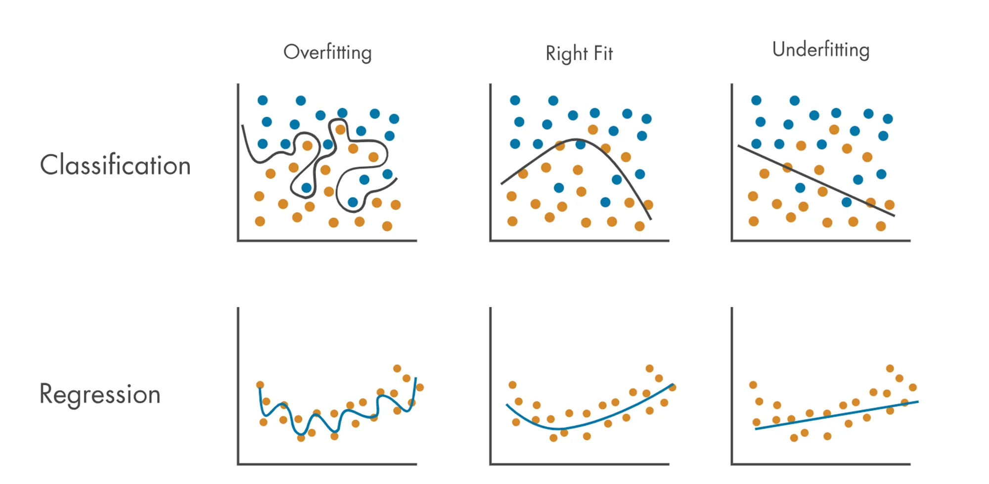
-
예측 혹은 분류를 하기 위해서 모형을 복잡도를 설정
- 모형이 지나치게 복잡할 때 → 과대 적합이 될 수 있음
- 모형이 지나치게 단순할 때 → 과소 적합이 될 수 있음
-
과적합의 원인
- 모델의 복잡도(상기의 예시)
- 데이터 양이 충분하지 않음
- 학습 반복이 많음(딥러닝의 경우)
- 데이터 불균형(정상환자 - 암환자의 비율이 95: 5)
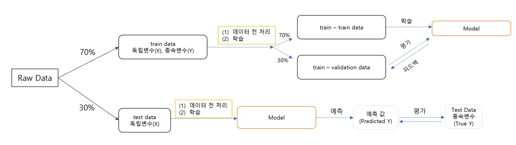
과적합 해결: 테스트 데이터의 분리
시험을 잘 보는 방법은 무엇일까요? 책뿐 아니라 모의고사를 열심히 풀어보는 방법이 아닐까요?
따라서, 한 데이터에서 테스트 데이터를 분리하여 모델에 학습시키는 방법을 사용하게 되었습니다.
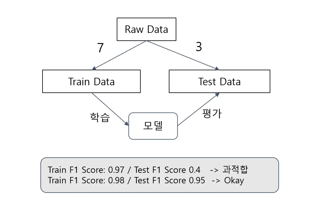
-
학습 데이터(Train Data): 모델을 학습(
fit)하기 위한 데이터 -
테스트 데이터(Test Data): 모델을 평가하기 위한 데이터
-
함수 및 파라미터 설명
- 함수
:sklearn.model_selection.train_test_split - 파라미터
test_size: 테스트 데이터 세트 크기train_size: 학습 데이터 세트 크기shuffle: 데이터 분리 시 섞기random_state: 호출할 때마다 동일한 학습/테스트 데이터를 생성하기 위한 난수 값 → 수행할 때 마다 동일한 데이터 세트로 분리하기 위해 숫자를 고정 시켜야 함!
- 반환 값(순서 중요!)
X_train,X_test,y_train,y_test
- 함수
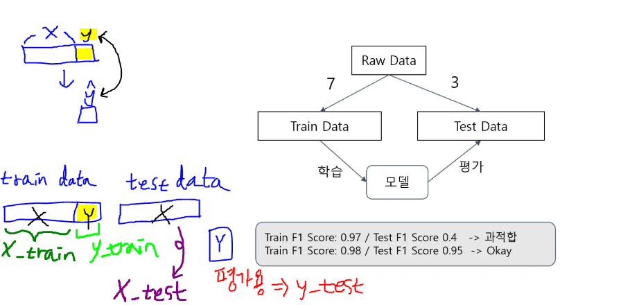
# train_test_split
# X 변수: Fare, Sex, Y 변수: Servived
from sklearn.model_selection import train_test_split
X_train, X_test, y_train, y_test = train_test_split(titanic_df[["Fare", "Sex"]], titanic_df[["Survived"]]
                                                    , test_size=0.3, shuffle=True, random_state=42)
print(f"X_train shape: {X_train.shape}, X_test shape: {X_test.shape}, y_train shape: {y_train.shape}, y_test shape: {y_test.shape}")
→ 실행 결과:
X_train shape: (623, 2), X_test shape: (268, 2), y_train shape: (623, 1), y_test shape: (268, 1)
# 원자료(raw data) 891개 Y값의 분포
sns.countplot(titanic_df, x="Survived")
sns.countplot(y_train, x="Survived")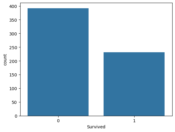
sns.countplot(y_test, x="Survived")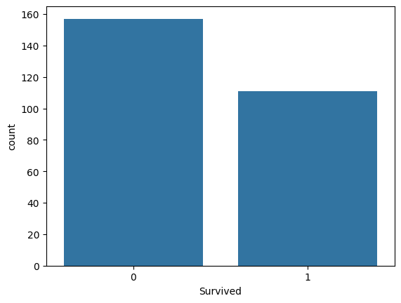
🡆 Raw Data의 생존자/사망자 비율이 y_train, y_test에서 모두 동일해야 좋은 split → 설정하는 option이 따로 있음: stratify(층화추출)
X_train, X_test, y_train, y_test = train_test_split(titanic_df[["Fare", "Sex"]], titanic_df[["Survived"]]
                                                    , test_size=0.3, shuffle=True, random_state=42, stratify=titanic_df[["Survived"]])
print(f"X_train shape: {X_train.shape}, X_test shape: {X_test.shape}, y_train shape: {y_train.shape}, y_test shape: {y_test.shape}")
※ 주의사항:
Test Data는 격리시켜두어야 함!
🡆 스케일링도 Train Data에 하고 그걸 Test로 가져와야지 원본에서 스케일링 학습 한 뒤 둘 다에 적용하면 안 된다고 함
실습: 데이터 분석 프로세스 전체 적용
- 데이터 로드 & 분리
- train / test 데이터 분리
- 탐색적 데이터 분석(EDA)
- 분포확인 & 이상치 확인
- 데이터 전처리
- 결측치 처리
- 수치형: Age
- 범주형: Embarked
- 삭제 : Cabin, Name
- 전처리
- 수치형: Age, Fare, Sibsp+Parch
- 범주형
- 레이블 인코딩: Pclass, Sex
- 원- 핫 인코딩: Embarked
- 결측치 처리
- 모델 수립
- 평가
train
import pandas as pd
import numpy as np
import seaborn as sns
import matplotlib.pyplot as plt

train_df = pd.read_csv("train.csv")
test_df = pd.read_csv("test.csv")

train_df.info()
→ Age, Embarked: NULL값 처리
→ Cabin: 삭제
train_df.describe(include="all")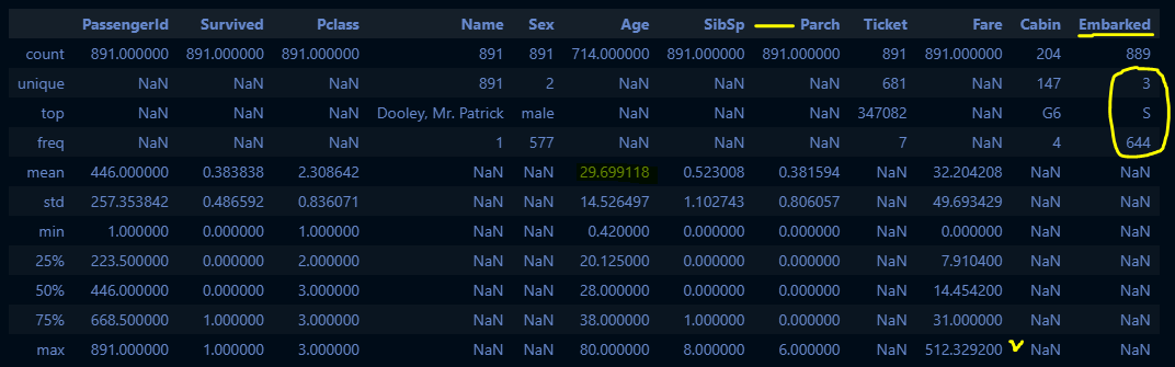
# 기초 가공: Family 변수 생성
train_df_2 = train_df.copy()
def get_family(df):
    df["Family"] = df["SibSp"] + df["Parch"] + 1
    df.drop(["SibSp", "Parch"], axis=1, inplace=True)
    return df
get_family(train_df_2).head(3)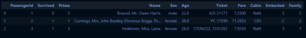
# pairplot으로 숫자형 변수들의 이상치 확인
sns.pairplot(train_df_2[["Age", "Fare", "Family"]])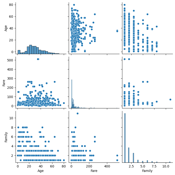
# Fare가 512를 넘는 값은 이상치로 보고 처리 및 인덱스 번호 리셋
train_df_2 = train_df_2[train_df_2["Fare"] < 512].reset_index(drop=True)
train_df_2.shape
(888, 11)
train_df_2.describe()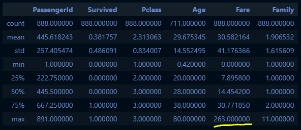
# 결측치 처리
def get_non_missing(df):
    Age_mean = train_df_2["Age"].mean()
    df["Age"] = df["Age"].fillna(Age_mean)

    # train 데이터에서는 필요하지 않지만 test 데이터에서 필요해서 추가
    Fare_mean = train_df_2["Fare"].mean()
    df["Fare"] = df["Fare"].fillna(Fare_mean)

    df["Embarked"] = df["Embarked"].fillna('S')
    return df

get_non_missing(train_df_2).info()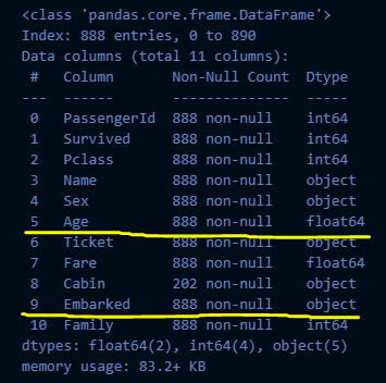
# 수치형 데이터 전처리
def get_numeric_sc(df):
    # std_sc: Fare, mm_sc: Age, Family
    from sklearn.preprocessing import StandardScaler, MinMaxScaler
    std_sc = StandardScaler()
    mm_sc = MinMaxScaler()

    std_sc.fit(train_df_2[["Fare"]])
    df["Fare_std_sc"] = std_sc.transform(df[["Fare"]])

    mm_sc.fit(train_df_2[["Age", "Family"]])
    df[["Age_mm_sc", "Family_mm_sc"]] = mm_sc.transform(df[["Age", "Family"]])

    return df

get_numeric_sc(train_df_2).describe()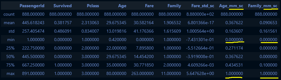
# 범주형 데이터 전처리
def get_categorical_encoding(df):
    from sklearn.preprocessing import LabelEncoder, OneHotEncoder
    le_Pclass = LabelEncoder()
    le_Sex = LabelEncoder()
    oe = OneHotEncoder()

    le_Pclass.fit(train_df_2[["Pclass"]])
    df["Pclass_le"] = le_Pclass.transform(df["Pclass"])

    le_Sex.fit(train_df_2[["Sex"]])
    df["Sex_le"] = le_Sex.transform(df["Sex"])

    oe.fit(train_df_2[["Embarked"]])
    embarked_csr = oe.transform(df[["Embarked"]])
    embarked_csr_df = pd.DataFrame(embarked_csr.toarray(), columns = oe.get_feature_names_out())
    df = pd.concat([df, embarked_csr_df], axis=1)

    return df

get_categorical_encoding(train_df_2).head(3)
train_df_2.info()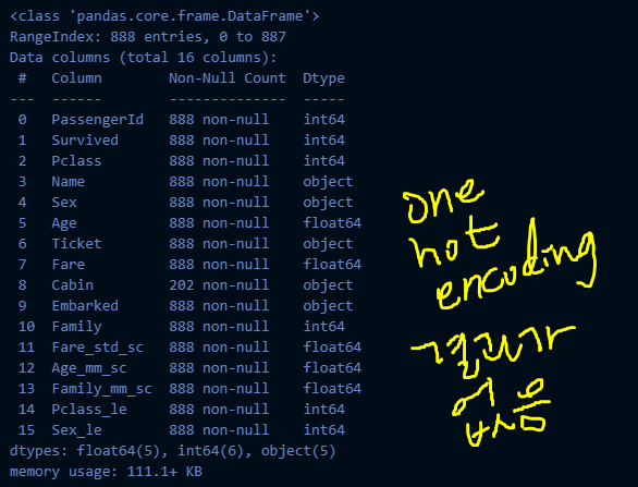
train_df_2 = get_categorical_encoding(train_df_2)
train_df_2.info()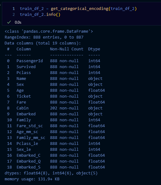
def get_model(df):
    from sklearn.linear_model import LogisticRegression
    model_lor = LogisticRegression()
    X = df[["Age_mm_sc", "Fare_std_sc", "Family_mm_sc", "Pclass_le", "Sex_le", "Embarked_C", "Embarked_Q", "Embarked_S"]]
    y = df["Survived"]

    return model_lor.fit(X, y)

model_lor_output = get_model(train_df_2)

X = train_df_2[["Age_mm_sc", "Fare_std_sc", "Family_mm_sc", "Pclass_le", "Sex_le", "Embarked_C", "Embarked_Q", "Embarked_S"]]
y_pred = model_lor_output.predict(X)

# 평가
from sklearn.metrics import accuracy_score, f1_score
print("accuracy score:", accuracy_score(train_df_2["Survived"], y_pred))
print("f1 score:", f1_score(train_df_2["Survived"], y_pred))
→ 실행 결과:
accuracy score: 0.8029279279279279
f1 score: 0.7320061255742726
test
# test 데이터로 적용하기
test_df.head(3)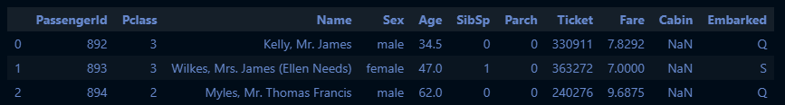
test_df.info()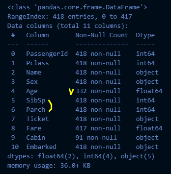
test_df_2 = get_family(test_df)
test_df_2.info()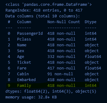
test_df_2 = get_non_missing(test_df_2)
test_df_2.info()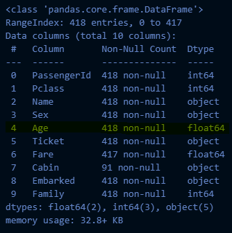
test_df_2 = get_numeric_sc(test_df_2)
test_df_2.info()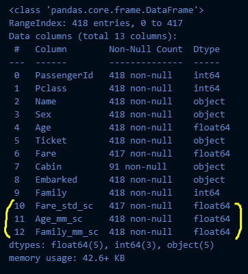
test_df_2 = get_categorical_encoding(test_df_2)
test_df_2.info()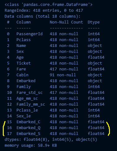
# get_model은 이미 만들어 놓은 model_lor_output을 사용해야 함
type(model_lor_output)
→ 실행 결과:
sklearn.linear_model._logistic.LogisticRegression
print(f"classes_:{model_lor_output.classes_}")
print(f"coef_:{model_lor_output.coef_}")
print(f"intercept_:{model_lor_output.intercept_}")
→ 실행 결과:
classes:[0 1]
coef:[[-2.18271749 -0.02718663 -1.24312952 -1.07248394 -2.59273756 0.17380464
0.10792882 -0.27513801]]
intercept_:[3.5130964]
X_test = test_df_2[["Age_mm_sc", "Fare_std_sc", "Family_mm_sc", "Pclass_le", "Sex_le", "Embarked_C", "Embarked_Q", "Embarked_S"]]
y_test_pred = model_lor_output.predict(X_test)

# model_lor_output.predict(X_test) 값을 Kaggle에 제출하면 결과 알려줌
sub_df = pd.read_csv("gender_submission.csv")
sub_df["Survived"] = y_test_pred
sub_df.to_csv("./result.csv", index=False)
교차 검증과 GridSearch
교차 검증(Cross Validation)
위에서 모델을 평가하기 위한 별도의 테스트 데이터로 평가하는 과정을 알아보았어요. 하지만 이때도, 고정된 테스트 데이터가 존재하기 때문에 과적합을 취약한 단점이 있답니다. 이를 피하기 위해서 교차검증방법 에 대해서 알아보아요.
- 교차검증(Cross Validation)
- 데이터 셋을 여러 개의 하위 집합으로 나누어 돌아가면서 검증 데이터로 사용하는 방법
K-Fold Validation
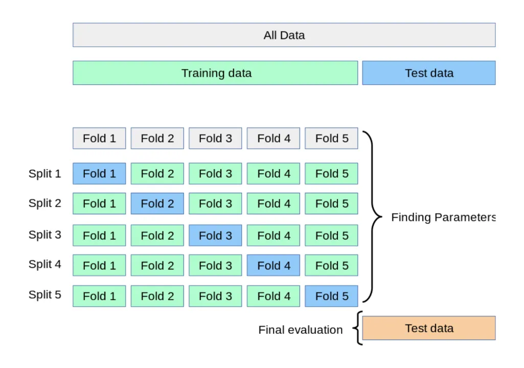
- 정의
- Train Data를 K개의 하위 집합으로 나누어 모델을 학습시키고 모델을 최적화 하는 방법
- K는 분할의 갯수
- Split 1: 학습용(Fold 2~5), 검증용(Fold1)
- Split 2: 학습용(Fold1, 3~5), 검증용(Fold2)
- Split 5까지 반복 후 최종 평가
- 특징
- 데이터가 부족할 경우 유용(반복 학습)
- 함수
skelarn.model_selection.KFoldsklearn.model_selection.StrifiedKFold- 불균형한 레이블(Y)를 가지고 있을 때 사용
# K fold 수행하기
from sklearn.model_selection import KFold

k_fold = KFold(n_splits=5)
scores = []
X = train_df_2[["Age_mm_sc", "Fare_std_sc", "Family_mm_sc", "Pclass_le", "Sex_le", "Embarked_C", "Embarked_Q", "Embarked_S"]]
y = train_df_2["Survived"]
for i, (train_index, test_index) in enumerate(k_fold.split(X)):
    X_train, X_test = X.values[train_index], X.values[test_index]
    y_train, y_test = y.values[train_index], y.values[test_index]

    from sklearn.linear_model import LogisticRegression
    from sklearn.metrics import accuracy_score
    model_lor_kfold = LogisticRegression()
    model_lor_kfold.fit(X_train, y_train)
    y_pred_kfold = model_lor_kfold.predict(X_test)
    accuracy = accuracy_score(y_test, y_pred_kfold)
    print(f"{i}번째 교차 검증 정확도는 {round(accuracy, 3)}")
    scores.append(round(accuracy, 3))

print(f"평균 정확도는 {np.mean(scores)}")
GridSearchV: 하이퍼 파라미터 자동 적용
알고리즘 심화에서 배울 내용이지만, 미리 알려드리자면 모델을 구성하는 입력 값 중 사람이 임의적으로 바꿀 수 있는 입력 값이 있습니다. 이를 하이퍼 파라미터(Hyper Parameter)라고 합니다. 다양한 값을 넣고 실험할 수 있기 때문에 이를 자동화해주는 Grid Search를 적용해볼 수 있습니다.
# GridSearch 적용하기
from sklearn.model_selection import GridSearchCV

params = {
    "solver": ["newton-cg", "lbfgs", "liblinear", "sag", "saga"]
    , "max_iter": [100, 200]
}
grid_lor = GridSearchCV(model_lor_kfold, param_grid=params, scoring="accuracy", cv=5)
grid_lor.fit(X_train, y_train)

print("최고의 하이퍼 파라미터", grid_lor.best_params_)
print("최고의 정확도", grid_lor.best_score_.round(3))
→ 실행 결과:
최고의 하이퍼 파라미터 {'max_iter': 100, 'solver': 'newton-cg'}
최고의 정확도 0.785
정리
숨 가쁘게 데이터 분석 전체 프로세스를 알아보았어요.
새로운 개념을 배울 때 메타 인지가 중요하기 때문에 데이터 분석 프로세스를 정리해볼게요.
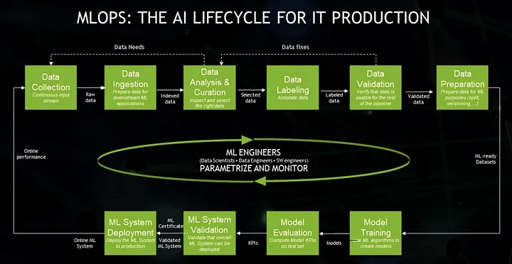
☞ 전체 데이터 프로세스
🡆 MLOps(머신러닝 작업)
개발과 운영을 따로 나누지 않고 개발의 생산성과 운영의 안정성을 최적화하기 위한 문화이자 방법론이 DevOps이며, 이를 ML 시스템에 적용한 것이 MLOps이다.
MLOps란 단순히 ML 모델뿐만 아니라, 데이터를 수집하고 분석하는 단계(Data Collection, Ingestion, Analysis, Labeling, Validation, Preparation), 그리고 ML 모델을 학습하고 배포하는 단계(Model Training, Validation, Deployment)까지 전 과정을 AI Lifecycle로 보고, MLOps의 대상으로 보고 있다.
ML에 기여하는 Engineer들(Data Scientist, Data Engineer, SW Engineer)이 ML의 전체 Lifecycle를 관리해야 한다.