Runge-Kutta 4th Model in MATLAB

20204.01.10

Runge-Kutta 4th method

🧐 Why do we use it?

: used in temporal discretization for the approximate solutions of simultaneous nonlinear equations

nonlinear equation에서 이산화를 통해 근사화시킨 결과를 얻는 방법.
즉, 근사화 방식을 통해 분석하는 numerical method 중 하나로 4차 룽게쿠타 방식이 가장 많이 사용된다.

🧐 How can we use it?

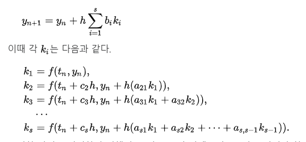
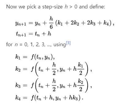
: 우리는 다음과 같은 수식을 이용하여 Runge-kutta 방식을 이용한다. 즉 y(n)의 결과값을 토대로 y(n+1)을 근사화시키는데, 이때 고정된 step size h와 가중치 값을 곱하여 사용하게 된다. 가중치는 k1~kn으로 나타나고 RK의 차수에 따라 그 개수가 정해진다. 우리가 사용하는 RK4 방식에서는 k1~k4까지의 가중치를 사용하게 되고, 보통의 step size는 0.001~0.01정도의 수치를 사용하게 된다.

이때, 가중치를 사용하지 않고 step size에만 의존하여 근사화시키는 방식을 'Euler's law'라고 한다. 가중치 없이 사용되기 때문에 step size가 크면 오차가 심하게 발생하는 결과를 가져온다.

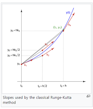
▸ we can check in 'Euler's law' we only uses h*f(t,w) term while Runge-Kutta 4th uses four different slopes to reduce the error. if we use too small step size for the accuracy, its process takes too much time for calculation. → instead runge kutta method suggests the effective ways for improving accuracy while using the similar time duration.

: h의 사이즈를 정확도를 위해 너무 줄이게 되면, 그에 trade off로 계산 시간이 많이 소모된다는 뜻이다. 이를 해결하는 방법이 4개의 가중치를 사용하는 Runge-kutta 4th method라는 것이다. 비슷한 시간을 소요하더라도 그 정확도는 오일러 법칙보다도 월등하게 개선한다.

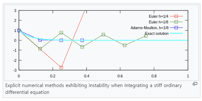
▸ Moreover, there’s one more way to express the method, which is ‘implicit Runge-Kutta’. It is used to cover the unstability of the explicit one. Implicit method is used for stiff equation, which is a differential equation for which certain numerical methods for solving the equation are numerically unstable, unless the step size is taken to be extremely small. In order for a numerical method to give a reliable solution to the differential system sometimes the step size is required to be at an unacceptably small level in a region where the solution curve is very smooth. The phenomenon is known as stiffness.

또한, 각각의 방법에는 implicit한 방식과 explicit한 방식이 있는데, 이는 stability 관점에서 바라보아야 한다. 보통 사용하는 것은 현재의 값을 토대로 다음 스탭의 값을 근사화시키는 explicit 방식이라면, implicit의 경우 현재의 값 뿐만 아니라 다음 스텝의 값 역시 다음 스텝의 값을 근사화 시키기 위한 수식에 포함된다.

이렇게 사용하면, 계산에 시간 소요가 굉장히 늘어나지만 그에 반해 explicit 한 것의 불안정성을 cover할 수 있다는 장점이 있다. 가끔은 step size를 불가능할 정도로 줄이지 않는 이상 발산하거나 정확하지 않는 수치로 근사화 되는 경우의 equation이 존재하는데, 그때는 explicit한 방법이 아닌 implicit한 방식을 사용하여 값을 정밀하게 근사화하여 찾을 수 있도록 한다.

[ MATLAB Simulation ]

% State space simulation with Runge-Kutta 4th method
% Matrix A is given and x is sol for homogeneous state eq
close all
clear
clc

% Define the time and h
h = 0.01;            % fixed step size
tfinal = 20;
t = 0: h: tfinal;     % time with h interval
x = [2; 3; 4];
x_out = zeros(3,length(t));

for n = 1:length(t)
    k1 = RK(t,x);
    k2 = RK(t+h/2, x+h*k1/2);
    k3 = RK(t+h/2, x+h*k2/2);
    k4 = RK(t+h, x+h*k3);
    
    x = x+(h/6)*(k1+2*k2+2*k3+k4); % Save the output
    x_out(:,n) = x;
end

plot(t,x_out(1,:))  % plot x1(t)
hold on
plot(t,x_out(2,:))  % plot x2(t)
plot(t,x_out(3,:))  % plot x3(t)

legend('x1','x2','x3')
xlabel('time')
title('Space state model using RK4')


% Define the function
% given matrix A is [0 1 0; 0 0 1; -2 -1 -5]
function y = RK(t,x)     
y = zeros(3,1);
y=[x(2); x(3); -2*x(1)-x(2)-5*x(3)];
end

A=[0 1 0; 0 0 1; -2 -1 -5] 라고 주어졌을 때, Runge-kutta 4th 방식을 이용하여 설계한 코드이다. 이때 matrix 연산을 바로 넣지 않고, function에 직접 A*x 를계산한 matrix를 삽입하였다. 이는 연산식이 복잡해지면 새로운 함수를 정의하여 matrix의 연산식을 그대로 넣는 것으로 대체할 수 있다. (뒤에서 다룰 예정.)

결과를 plot하면 다음과 같다.

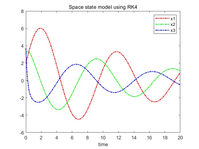
(for time 20sec)

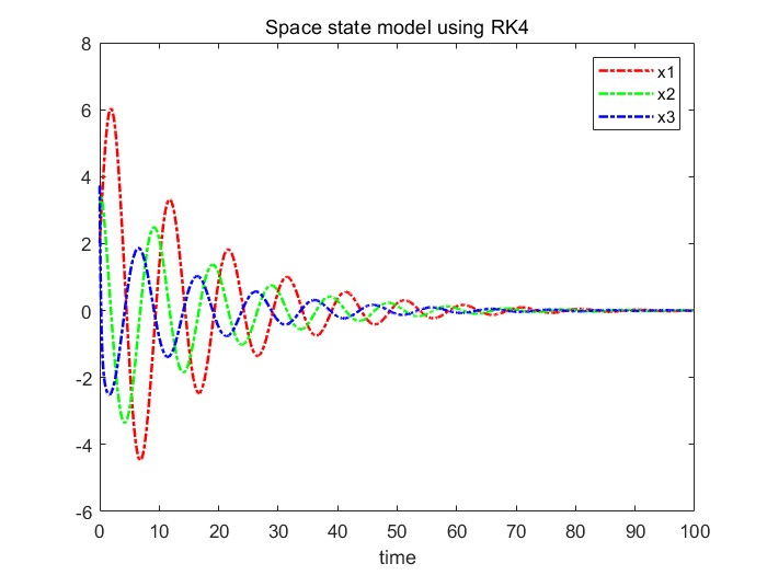
(for time 100sec)

❓ 이때 궁금증이 하나 생긴다.
A matrix를 A'으로 바꾸고 plot하면 어떤 변화가 생길까?

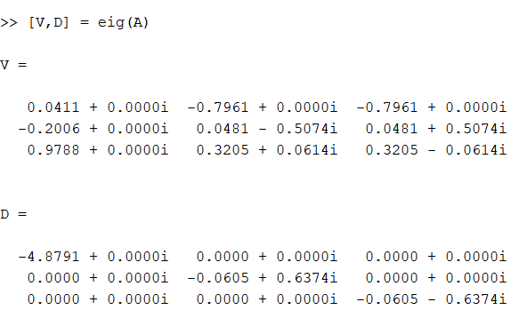
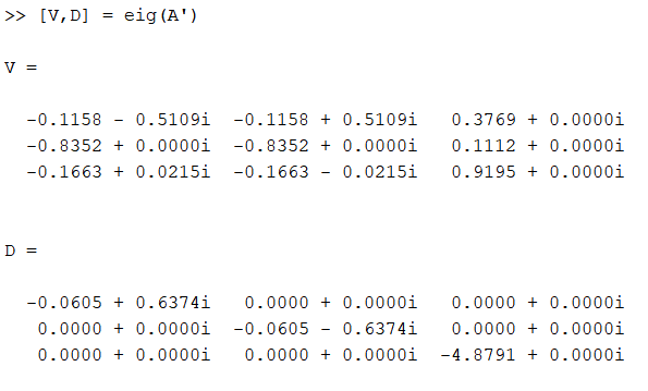
A와 A 전치 행렬의 eigen value는 같다. 그렇다면 eigen valuse가 같은 행렬의 연산은 homogeneous eq의 solution은 plot하면 같은 결과가 나와야 하지 않을까?

실제로 matrix를 전치행렬로 바꾸고 시행하면 결과는 다음과 같다.

% Define the function
% given matrix A is [0 0 -2; 1 0 -1; 0 1 -5] (A transpose)
function y = RK(t,x)     
y = zeros(3,1);
y=[-2*x(3); x(1)-x(3); x(2)-5*x(3)];
end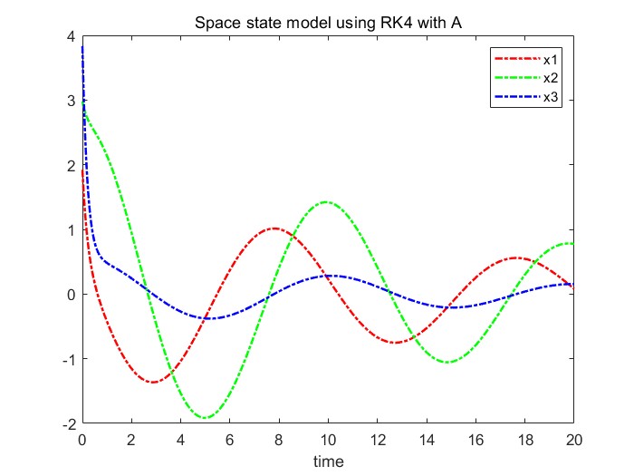

실제 결과값을 보면 x1~x3까지 차이가 발생하는 것을 볼 수 있다. 이에 대한 이유를 찾아보면 다음과 같은 해답을 얻을 수 있었다.
"A와 A’의 eigen value는 같기 때문에 초기값과 미분방정식의 형태에만 의존하여 해를 구하는 Runge-Kutta 방법으로 구한 해의 값은 같아야 하지만, 고유값이 같아도 고유 벡터가 다른 경우 해가 다르게 나올 수 있다. 실제로 A와 A’의 고유 벡터값을 구하면 아래와 같다."

❓ 이번엔 또다른 궁금증.
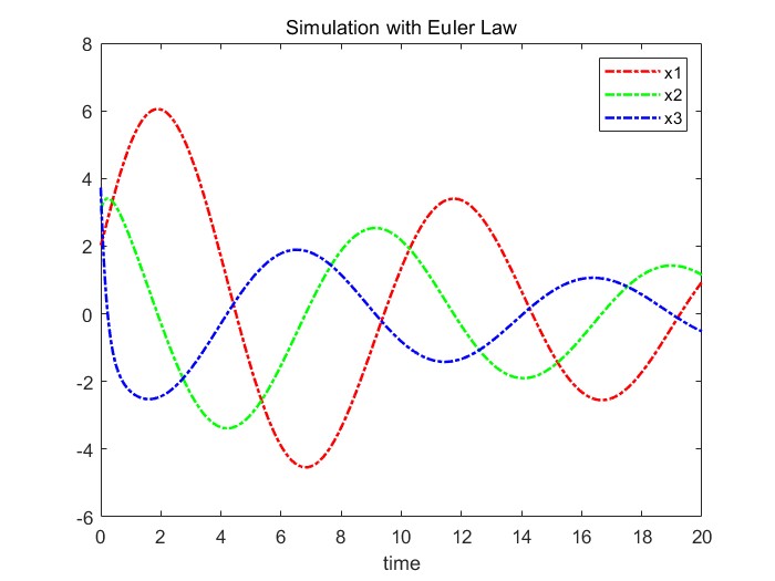
그렇다면 Euler's law로 plot한 결과와 Runge-Kutta 4th의 방식은 얼마나 차이가 발생할까?

이번엔 오일러법칙을 이용하여 plot하고 그 결과를 그래프로 비교해본다.

% State space simulation with Euler's law
% Matrix A is given and x is sol for homogeneous state eq

close all
clear
clc


% Define the time and h
h = 0.01;                       % fixed step size
tfinal = 20;
t = 0: h: tfinal;               % time with h interval
x = [1; 1; 1];                  % initial value
x_out = zeros(3,length(t));     % save output as the column vector

for n = 1:length(t)
    x = x+h*EU(t,x);  % Save the output
    x_out(:,n) = x;

end

figure(2);
plot(t,x_out(1,:),'r')  % plot x1(t)
hold on
plot(t,x_out(2,:),'g')  % plot x2(t)
plot(t,x_out(3,:),'b')  % plot x3(t)


legend('x1','x2','x3')
xlabel('time')
title('Space-state model using Euler''s law')

% Define the function
% given matrix A is [0 1 0; 0 0 1; -2 -1 -5]
function y = EU(t,x)      
y = zeros(3,1);
y=[x(2); x(3); -2*x(1)-x(2)-5*x(3)];
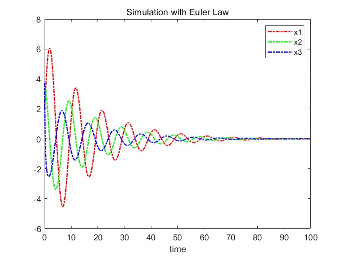
end

오일러 법칙을 20초간 simulation해보면 다음과 같은 결과를 얻을 수 있다.

또한, 40초 동안 simulation해보면 수렴하는 양상을 더 잘 관찰할 수 있는데, 이는 다음 사진과 같다.

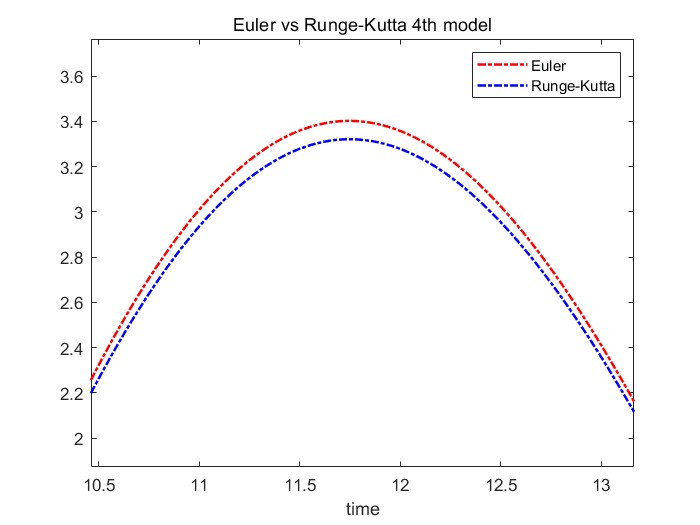
이를 Runge Kutta 4th 방식과 비교해보면 다음과 같다. 20초 동안 동일하게 Euler's law와 Runge-kutta 방식을 plot해보면 거의 비슷하게 나오는 것을 볼 수 있다.

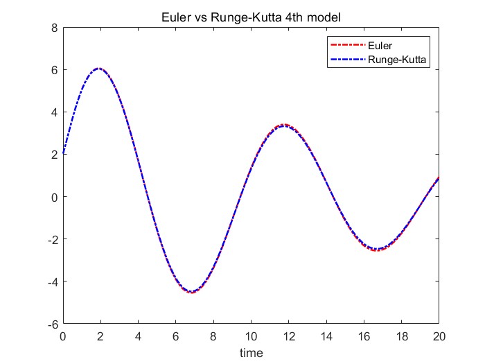
이를 확대하여 발생하는 오차를 보면, Euler과 Runge-kutta 사이에 오차가 발생하는 것을 확인해볼 수 있다.