2024.01.17
Complex Plane
: geometric representation of complex numbers. By using the complex plane, we can represent the complex number as the vector.

› 감쇠비 (ζ) : 시스템이 얼마나 빨리 혹은 천천히 진동을 멈출지를 나타낸다. 감쇠비가 작을 수록 (0에 가까울 수록) 시스템은 빠르게 진동, 클수록 (1에 가까울 수록) 진동이 빨리 멈춘다. 감쇠비가 1보다 크면 시스템이 overdamping 상태로, 진동이 빨리 멈춘다.
› 감쇠율(Decay rate σ) : 시스템이 초기조건에서 출발하여 얼마나 빨리 안정상태로 수렴하는지를 나타낸다. 이는 감쇠비와 자연주파수로 나타내고, 감쇠율이 양수면 진동이 감쇠되어 시간이 흐름에 따라 진폭이 감소함을 나타낸다.
› 감쇠 주파수(ωd) : 감쇠된 진동의 주파수. 감쇠율과 자연주파수를 이용해 표현되는 식. 감쇠율이 증가하면 감쇠된 주파수는 감소한다.
› 자연주파수(ωn) : 시스템이 자유진동할 때의 진동 주파수(외부의 driving 혹은 damping 힘이 없을 때를 나타낸다). 이때 자연주파수의 제곱은 k(스프링 상수/시스템의 탄성)에 비례하고, m(시스템의 질량)에 반비례한다. 자연주파수는 진동하는 속도에 영향을 미치는데, 높은 자연 주파수는 짧은 진동 주기를 의미함.
State feedback controller
: A method used in feedback control system theory to place the closed-loop poles of a plant in the pre-determined locations in the s-plane. Placing poles are directly related to the eigenvalue → eigenvalue controls the characteristics of the response of the system.

→ Full state feedback is utilized by commanding the input vector u. Consider an input proportional to the state vector (x). (u = r(t)-Kx(t))
Desired poles

1. sys의 response에 pole 뿐만 아니라 zero도 영향을 미침을 고려해야 한다.
2. Im축과 평행한 직선 → 멀리 떨어질수록 response 속도가 빠르다.
3. 음수 Real축과 Imaginary 축이 이루는 각 theta → 각도가 클수록 Mp(overshoot)가 크다.
4. 한 곳에 모든 eigen value가 있거나, 가까이 모여있으면 → 응답은 느리고, actuating signal 크기가 크다. (bad 😐 → actuating(input) signal이 크면 물리적 시스템이 타거나 saturate될 수 있음에 주의해야 한다.)
위 사항들을 고려하여 system이 원하는 사양을 가질 수 있도록 pole을 설정한다.
Design State-Estimator
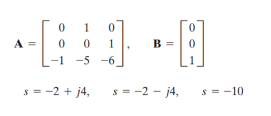
주어진 desird pole을 가지는 state-estimator 설계 (코드 일부)
% Establish the controller with pole placement

% define the matrix (state space)
A=[0 1 0; 0 0 1; -1 -5 -6];
B=[0; 0; 1];
p=[-2+4j -2-4j -10];    % desired poles

k=place(A,B,p);         % find the feedback gain k
이를 plot한 결과는 아래와 같다.
(1) State-estimator 없이 Runge-Kutta 4th만 이용한 open loop system

(2) State-estimator을 설치하여 Runhe-Kutta 4th를 이용한 Clsoed loop system

이를 보면, Closed loop을 만들어 plot한 결과 open loop에 비해 빠른 속도로 0으로 수렴하는 것을 볼 수 있다. (빠른 속도로 안정화 되는 것을 볼 수 있다.)
Filter (Observer)
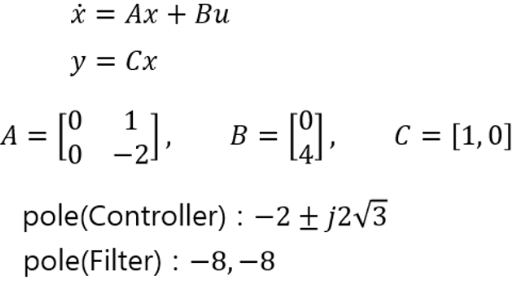
이번엔 위의 desired pole을 가진 state-controller과 그보다 4배 멀리 떨어져 빠르게 수렴하도록 하는 observer pole을 가진 system을 구성해본다.
% Desired poles for the controller
p_controller=[-2+2j*sqrt(3) -2-2j*sqrt(3)];    % Desired poles
k=acker(A,B,p_controller);                     % Find with pole placement
% Desired poles for the filter
p_filter=[-8 -8];                              % Desired poles for the filter
ke=acker(A',C',p_filter);                      % Use Duality (Acker vs place?)

% DE becomes x'=(A-Bk-ke'C)x+ke*y
A_f = A-B*k-ke'*C;
acker함수를 controller을 이용할 때 k값을 찾기 위해 사용한 것처럼, observer 역시 dual system을 이용하여 동일한 방식으로 acker함수를 사용하여 ke 값을 찾는다. 이후의 과정은 동일한 Runger-Kutta 방식으로 마무리 하면 된다.
✔ 이번엔 simulink를 이용해보자.
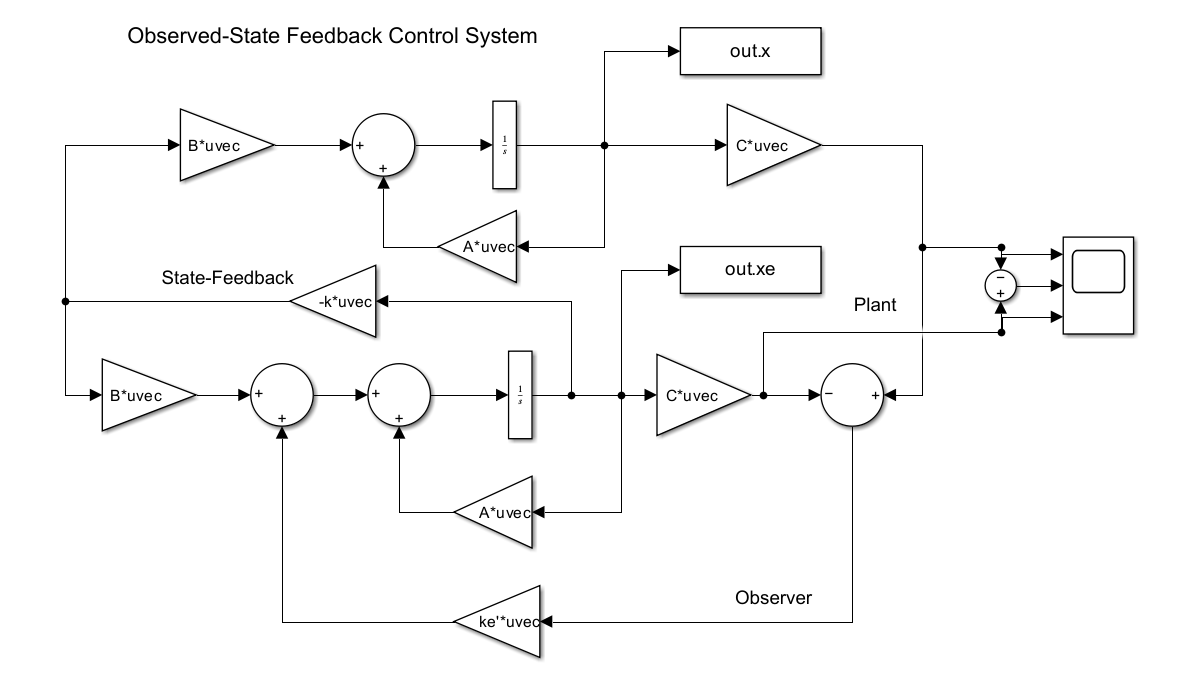
< Simulink Steady-State Design>
이번에는 simulink에서 추출한 x_out과 상태 추정값인 xe_out값을 이용하여 error값을 출력할 것이다. 이에 의해 우리는 system이 안정화 되는 것을 관찰하고, xe의 추정값이 실제 x값을 잘 따라가는지,즉 error이 0으로 잘 수렴하는 지 확인 할 것이다.

<Scope를 통해 확인한 x,xe에 대한 error>
이러한 x, xe, error값을 통해 matlab에서 plot한 결과는 다음과 같다. 아래는 이에 대한 matlab 코드와 plot 결과이다.
% Establish Controller
close all
clear
clc
%%

% Define steady state sys
A=[0 1; 0 -2];
B=[0;4];
C=[1 0];
D=0;

% Desired poles for the controller
p_controller=[-2+2j*sqrt(3) -2-2j*sqrt(3)];    % Desired poles
k=acker(A,B,p_controller);                     % Find with pole placement
% Desired poles for the filter
p_filter=[-8 -8];                              % Desired poles for the filter
ke=acker(A',C',p_filter);                      % Use Duality (Acker vs place?)

out = sim('Observer_s.slx',10);
Time=out.x.time;
X=out.x.signals.values;
Xe=out.xe.signals.values;
Error = Xe-X;

fig1=figure(1);
subplot(2,1,1);
a1=plot(Time, X(:,1),'-.r','Linewidth', 1); hold on
a2=plot(Time, Xe(:,1),'-.b','Linewidth', 1); hold on
a3=plot(Time, Error(:,1),'-.k','Linewidth', 1); hold on
xlabel('time')
ylabel('state and estimation for X1')
legend([a1,a2,a3],{'$x_{1}$','$xe_{1}$','$error$'},'Interpreter','latex')
title('Observed-State Feedback Control System')

subplot(2,1,2);
a4=plot(Time, X(:,2),'-.r','Linewidth', 1); hold on
a5=plot(Time, Xe(:,2),'-.b','Linewidth', 1); hold on
a6=plot(Time, Error(:,2),'-.k','Linewidth', 1); hold on
xlabel('time');
ylabel('state and estimation for X2')
legend([a4,a5,a6],{'$x_{2}$','$xe_{2}$','$error$'},'Interpreter','latex')
이는 simulink에서 뽑아낸 x와 xe값을 그대로 사용하여 matlab에서 plot한 것이다.
✔ 아래의 부분이 바로 simulink에서 값을 가져오는 방식이니 꼭 참고!
out = sim('Observer_s.slx',10);
Time=out.x.time;
X=out.x.signals.values;
Xe=out.xe.signals.values;
Error = Xe-X;
이를 실제로 plot해보면 결과는 아래와 같다.

Discussion
› 초기조건에 따라 Xe가 X를 따라오는 차이가 발생한다. X 추정치는 실제 값을 따라오는데 초기값의 영향을 많이 받음을 알 수 있다. → 초기값 차이가 작으면 금방 따라오지만, 초기값 차이가 크면 따라오는데 오차가 상대적으로 크게 발생함.
› 시간이 지나면 Error (X-Xe)는 0으로 수렴함.