
📚 Multinomial Classification
저번 글에서 다룬 Multinomial Classification을 Iris Data Set을 이용하여 구현해보자. 이번에도 sklearn과 tensorflow를 사용하여 구현하고, classification_report 함수 (평가 함수)를 사용하여 검증까지 해보자.
import numpy as np
import pandas as pd
import matplotlib.pyplot as plt

from sklearn.datasets import load_iris

from scipy import stats
from sklearn.preprocessing import MinMaxScaler, StandardScaler
from sklearn.model_selection import train_test_split

from sklearn import linear_model
from tensorflow.keras.models import Sequential
from tensorflow.keras.layers import Flatten, Dense
from tensorflow.keras.optimizers import Adam
from tensorflow.keras.callbacks import EarlyStopping

from sklearn.metrics import classification_report
📚 classification_report
Model 구현으로 넘어가기 전에, classification_report 함수에 대해서 간단하게 알아보자. 이전에 사용했던 BMI Data Set을 예시로 사용할 것이다.
from sklearn.metrics import classification_report

# 정답 데이터와 예측 데이터가 있어야 한다.
# 0 : thin, 1 : normal, 2 : fat
t_data = [0, 1, 2, 2, 2] # 정답 데이터
predict = [0, 0, 2, 2, 1] # 모델의 예측 데이터
target_name = ['thin', 'normal', 'fat']
print(classification_report(t_data, predict, target_names=target_name))
#               precision    recall  f1-score   support

#         thin       0.50      1.00      0.67         1
#       normal       0.00      0.00      0.00         1
#          fat       1.00      0.67      0.80         3

#     accuracy                           0.60         5
#    macro avg       0.50      0.56      0.49         5
# weighted avg       0.70      0.60      0.61         5
이처럼 정답 데이터와 예측 데이터를 비교하여 Accuracy(정확도), Recall(재현율), Precision(정밀도), F1 Score 값을 계산해 준다.
📚 Data Preprocessing
sklearn에서 기본적으로 제공하는 Iris Data Set을 사용하여 Iris의 종류를 예측하는 모델을 구현해보자.
📚 Raw Data Loading
iris = load_iris()
df = pd.DataFrame(iris.data, columns=iris.feature_names)

df.columns = ['sepal_length', 'sepal_width', 'petal_length', 'petal_width']
df['label'] = iris.target

display(df.head())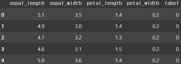
📚 결측치 확인 및 처리
df.isnull().sum()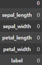
결측치는 존재하지 않는다.
📚 중복데이터 확인 및 처리
print(df.duplicated().sum()) # 1

df_new = df.drop_duplicates()
display(df_new.shape) # (150, 5) -> (149, 5)
의미 없이 중복된 데이터가 1개 존재하므로 drop_duplicates() 함수를 사용하여 간단하게 삭제 처리해주었다.
📚 상관관계 분석
print(df.corr())
#               sepal_length  sepal_width  petal_length  petal_width     label
# sepal_length      1.000000    -0.117570      0.871754     0.817941  0.782561
# sepal_width      -0.117570     1.000000     -0.428440    -0.366126 -0.426658
# petal_length      0.871754    -0.428440      1.000000     0.962865  0.949035
# petal_width       0.817941    -0.366126      0.962865     1.000000  0.956547
# label             0.782561    -0.426658      0.949035     0.956547  1.000000
우리는 주어진 데이터를 처리할 때 각 독립변수가 종속변수에 얼마나 영향을 미치는지 분석하고, 영향을 많이 미치지 않는 독립변수는 overfitting을 방지하기 위해 삭제할 필요가 있다. 이때 corr() 함수를 사용하여 상관계수를 출력해 볼 수 있는데, 이 값은 -1 ~ 1 (1은 양의 상관관계, -1은 음의 상관관계) 사이의 실수로 계산되며 양 극단으로 갈 수록 상관관계가 높다고 볼 수 있다.
📚 이상치 확인 및 처리
fig = plt.figure()
ax1 = fig.add_subplot(1, 4, 1)
ax2 = fig.add_subplot(1, 4, 2)
ax3 = fig.add_subplot(1, 4, 3)
ax4 = fig.add_subplot(1, 4, 4)

ax1.set_title('sepal_length')
ax2.set_title('sepal_width')
ax3.set_title('petal_length')
ax4.set_title('petal_width')

ax1.boxplot(df_new['sepal_length'])
ax2.boxplot(df_new['sepal_width'])
ax3.boxplot(df_new['petal_length'])
ax4.boxplot(df_new['petal_width'])

plt.tight_layout()

plt.show()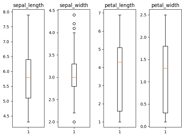
몇개의 이상치가 확인되지만 이 데이터는 실제 데이터이고, 이상치가 범위에서 크게 벗어나지 않으므로 삭제하지 않았다.
📚 데이터 정규화
x_data = df_new.drop('label', axis=1, inplace=False).values # 2차원
t_data = df_new['label'].values # 1차원

scaler = StandardScaler()
scaler.fit(x_data)
x_data_norm = scaler.transform(x_data)
분류 모델이므로 독립변수에 대해서만 정규화를 진행하였고, 이상치 처리를 따로 진행하지 않았기 때문에 Z-Score를 사용하는 Standardization을 사용하였다.
📚 데이터 분할
x_data_train_norm, x_data_test_norm, t_data_train, t_data_test = \
train_test_split(x_data_norm, t_data,
                 test_size=0.2, stratify=t_data)
평가를 진행하기 위해 데이터를 Training/Test Set으로 분할해준다. 이때 데이터가 부족하므로 test_size는 0.2로 일반적인 경우보다 적게 지정하였다.
📚 Multinomial Classification 구현 (sklearn)
sklearn_model = linear_model.LogisticRegression()
sklearn_model.fit(x_data_train_norm, t_data_train)
sklearn 내부적으로 One-Hot Encoding 처리하여 학습을 진행하기 때문에 1차원 t_data를 그대로 학습에 사용하였다.
📚 모델 평가
sklearn_result = sklearn_model.predict(x_data_test_norm)
print(classification_report(t_data_test, sklearn_result,
                            target_names=['Setosa', 'Vesicolor', 'Virsinica']))
#               precision    recall  f1-score   support

#       Setosa       1.00      1.00      1.00        10
#    Vesicolor       0.91      1.00      0.95        10
#    Virsinica       1.00      0.90      0.95        10

#     accuracy                           0.97        30
#    macro avg       0.97      0.97      0.97        30
# weighted avg       0.97      0.97      0.97        30
📚 Multinomial Classification 구현 (tensorflow)
keras_model = Sequential()

keras_model.add(Flatten(input_shape=(4,)))
keras_model.add(Dense(units=3, activation='softmax'))

keras_model.compile(optimizer=Adam(learning_rate=1e-1),
                    loss='sparse_categorical_crossentropy',
                    metrics=['acc'])

es_callback = EarlyStopping(monitor='val_loss', patience=5,
                            restore_best_weights=True, verbose=1)

keras_model.fit(x_data_train_norm, t_data_train.reshape(-1, 1),
                          epochs=1000, verbose=1,
                          validation_split=0.2, callbacks=[es_callback])
Multinomial Classification 모델이므로 활성화 함수로는 Softmax 함수를, One-hot Encoding 처리를 내부적으로 알아서 하기 위해 loss 함수로는 sparse_categorical_crossentropy 함수를 사용하였다.
또한 불필요한 반복으로 인해 overfitting되는 것을 방지하게 위해 EarlyStopping callback을 사용하여 validation loss가 5 epochs 동안 개선되지 않을 시 학습을 중단하도록 하였다.
📚 모델 평가
keras_result = keras_model.predict(x_data_test_norm)

# 2차원 확률값을 1차원 label값으로 변경
keras_result = np.argmax(keras_result, axis=1)

print(classification_report(t_data_test, keras_result,
                            target_names=['Setosa', 'Vesicolor', 'Virsinica']))
#               precision    recall  f1-score   support

#       Setosa       1.00      1.00      1.00        10
#    Vesicolor       0.91      1.00      0.95        10
#    Virsinica       1.00      0.90      0.95        10

#     accuracy                           0.97        30
#    macro avg       0.97      0.97      0.97        30
# weighted avg       0.97      0.97      0.97        30
tensorflow 모델의 Test Data Set에 대한 예측값은 2차원 데이터로 출력되기 때문에 (sklearn 모델과 다르게 입력이 2차원이기 때문에) classification_report 함수를 사용하기 위해 NumPy의 argmax() 함수를 사용하여 1차원 label 값으로 변경시켜주어야 한다.